A Look at The First Place Solution of a Dermatology Classification Kaggle Competition
One interesting thing I often think about is the gap between academic and real-world solutions. In general academic solutions play in the realm of idealized problem spaces, removing themselves from needing to care about the messiness of the real-world. Kaggle competitions are a (small) step in the right direction towards dealing with messiness, usually providing a true blind test set (vs. overused benchmarks), and opening a few degrees of freedom in terms the techniques that can be used, which usually eschews novelty in favour of more robust methods. To this end, I thought it would be useful to take a look at a more realistic problem (via a Kaggle competition) and understand the practical details that result in a superior solution.
This post will cover the first place solution [1] to the SIIM-ISIC Melanoma Classification [0] challenge. In addition to using tried and true architectures (mostly EfficientNets), they have some interesting tactics they use to formulate the problem, process the data, and train/validate the model. I'll cover background on the ML techniques, competition and data, architectural details, problem formulation, and implementation. I've also run some experiments to better understand the benefits of certain choices they made. Enjoy!
Table of Contents
1 Background
1.1 Inverted Residuals and Linear Bottlenecks (MobileNetV2)
MobileNetV2 [2] introduced a new type of neural network architectural building block often referred to as "MBConv". The two big innovations here are inverted residuals and linear bottlenecks.
First to understand inverted residuals, let's take a look at the basic
residual block (also see my post on ResNet)
shown in Listing 1. Two notable parts of the basic residual block are the
fact that we reduce the number of channels to squeeze in the first
layer, and then grow the number of channels to expand in the last
layer. The squeeze operation is often known as a bottleneck since we have
fewer channels. The intuition here is to reduce the number of channels so that
the more expensive 3x3 convolution is cheaper. The other relevant part is that
we have the residual "skip" connection where we add the input to the
result of the transformations. Notice the residual connection connects the
expanded parts x and m3.
def residual_block(x, squeeze=16, expand=64):
    # x has 64 channels in this example
    m1 = Conv2D(squeeze, (1,1), activation='relu')(x)
    m2 = Conv2D(squeeze, (3,3), activation='relu')(m1)
    m3 = Conv2D(expand, (1,1), activation='relu')(m2)
    return Add()([m3, x])
Listing 1: Example of a Basic Residual Block in Keras (adapted from source)
Next, let's look the changes in an inverted residual block shown in Listing 2. Here we "invert" the residual connection where we are making the residual connection between the bottleneck "squeezed" layers instead of "expanded" layers. Recall that we'll eventually be stacking these blocks, so there will still be alternations of squeezed ("bottlenecks") and expansion layers. The difference with Listing 1 is that we'll be making residual connections between the bottleneck layers instead of expansion layers.
def inverted_residual_block(x, expand=64, squeeze=16):
    # x has 16 channels in this example
    m1 = Conv2D(expand, (1,1), activation='relu')(x)
    m2 = DepthwiseConv2D((3,3), activation='relu')(m1)
    m3 = Conv2D(squeeze, (1,1), activation='relu')(m2)
    return Add()([m3, x])
Listing 2: Example of an inverted residual block with depthwise convolution in Keras (adapted from source)
The other thing to note is that the 3x3 convolution is now expensive if we do it on the expanded layer, so instead we'll use a depthwise convolution for efficiency. This reduces the number of parameters needed from \(h\cdot w \cdot d_i \cdot d_j \cdot k^2\) for a regular 3x3 convolution to \(h\cdot w \cdot d_i (k^2 + d_j)\) for a depthwise convolution where \(h, w\) are height and width, \(d_i, d_j\) are input/output channels, and \(k\) is the convolutional kernel size. With \(k=3\) this could potentially reduce the number of parameters needed by 8-9 times with only a small hit to accuracy.
def inverted_linear_residual_block(x, expand=64, squeeze=16):
    m1 = Conv2D(expand, (1,1), activation='relu')(x)
    m2 = DepthwiseConv2D((3,3),  activation='relu')(m1)
    m3 = Conv2D(squeeze, (1,1))(m2)
    return Add()([m3, x])
Listing 3: MBConv Block in Keras (adapted from source)
The last big thing thing that MBConv block changes was removing the non-linearity on the bottleneck layer as shown in Listing 3. A hypothesis the [2] proposes is that ReLU non-linearity on the inverted bottleneck hurts performance. The idea is that ReLU either is the identify function if the input is positive, or zero otherwise. In the case that the activation is positive, then it's simply a linear output so removing the non-linearity isn't a bit deal. On the other hand, if the activation is negative then ReLU actively discards information (e.g., zeroes the output). Generally for wide networks (i.e., lots of convolutional channels), this is not a problem because we can make up for information loss in the other channels. In the case of our squeezed bottleneck though, we have fewer layers so we lose a lot more information, hence hurt performance. The authors note that this effect is lessened with skip connections but still present. (Note: Not shown in the above code is that BatchNormalization is applied after every convolution layer (but before the activation).)
The resulting MobileNetV2 architecture is very memory efficient for mobile applications as the name suggests. Generally, the paper shows that MobileNetV2 uses less memory and computation with similar (sometimes better) performance on standard benchmarks. Details on the architecture can be found in [2].
1.2 Squeeze and Excitation Optimization
The Squeeze and Excitation (SE) block [3] is an optimization that can be added on to a convolutional layer that scales each channel's outputs by using a learned function of the average activation of each channel. The basic idea is shown in Figure 1 where from a convolution operation (\(F_{tr}\)), we branch off to calculate a scalar per channel ("squeeze" via \(F_{sq}\)), pass it through some layers ("excite" via \(F_{ex}\)), and then scale the original convolutional outputs using the SE block. This can be thought of as a self-attention mechanism on the channels.
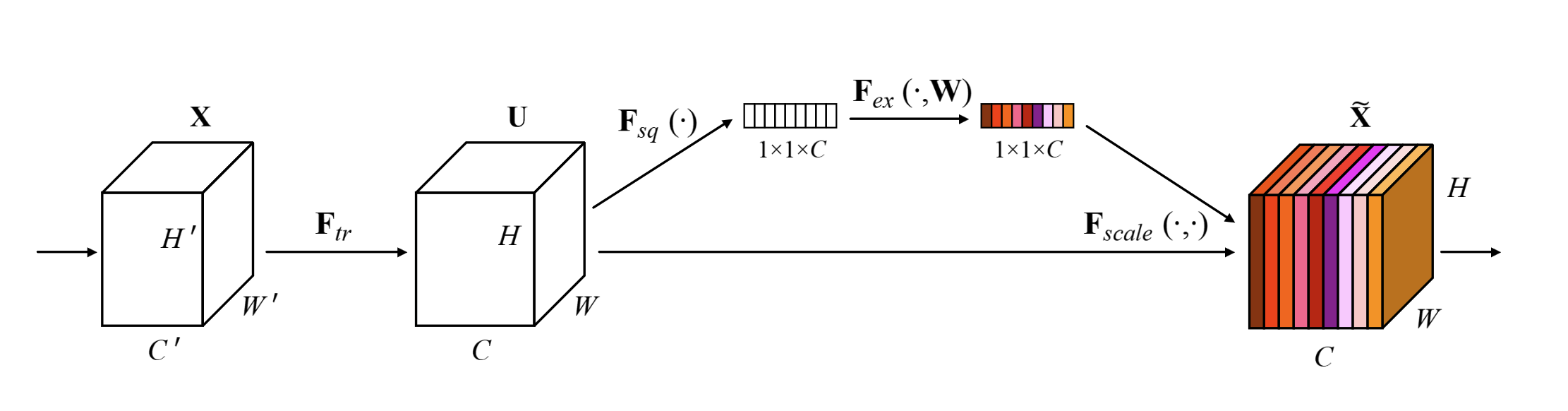
Figure 1: Squeeze Excitation block with ratio=1 [ 3 ]
The main problem the SE block addresses is that each convolutional output pixel only looks at it's local receptive field (e.g. 3x3). A convolutional network only really considers global spatial information by stacking multiple layers, which seems inefficient. Instead, the hypothesis of the SE block is that you can model the global interdependencies between channels and allow each channel to increase their sensitivity improving learning.
Code for an SE block is shown in Listing 4. First, we do a
GlobalAveragePool2D, which computes the mean for each
channel. Then we pass it through two 1x1 convolutional layers with a ReLU and
sigmoid activation respectively. The first convolutional layer can be thought
of as "mixing" the averages across the channels, while the second one converts
it to a value between 0 and 1. It's not clear whether more or less layers is better
but [3] says that they wanted to limit the added model complexity while still
having some generalization power.
def squeeze_excite(x, filters, ratio=4):
    # computes mean of each spatial dimensions (outputs a mean value for each channel)
    m1 = GlobalAveragePooling2D(keepdims=True)(x)
    m2 = Conv2D(filters // ratio, (1, 1), activation='relu')(m1)
    m3 = Conv2D(filters, (1, 1), activation='sigmoid')(m2)
    return Multiply(m3, x)
Listing 4: SqueezeExcite block in Keras (adapted from source)
Since the SE block only operates on channels as a whole, the added computational and memory requirements are modest. The largest contributors are usually the latter layers that have a lot of channels. In their experiments the parameters of a MobileNet network increased by roughly 12% but was able to improve the ImageNet top-1 error rate by about 3% [3]. Overall, it seems like a nice little optimization that improves performance across a wide variety of visual tasks.
1.3 EfficientNet
EfficientNet is a convolutional neural networks (ConvNet) architecture [4] (circa 2019) that rethinks the standard ConvNet architecture choices and proposes a new architecture family called EfficientNets. The first main idea is that ConvNets can be scaled to have more capacity in three broad network dimensions shown in Figure 2:
Wider: In the context of ConvNets, this corresponds to more channels per layer (analogous to more neurons in a fully connected layer).
Deeper: Corresponds to more convolutional layers.
Higher Resolution: Corresponds to using higher resolution inputs (e.g. 560x560 vs. 224x224 images).
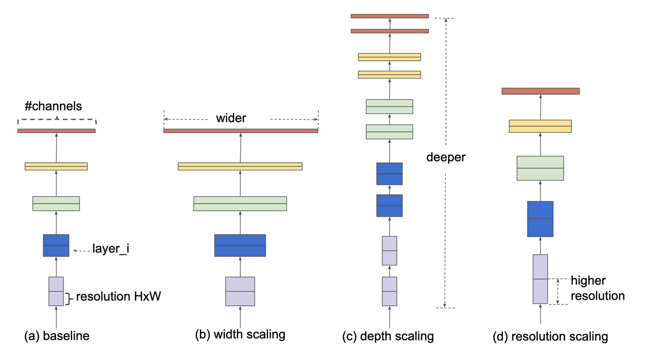
Figure 2: Model scaling figure from [ 4 ]: (a) base model, (b) increase width, (c) increase depth, (d) increase resolution.
The first insight [4] found is that, as expected, scaling the above network dimensions result in better ConvNet accuracy (as measured via top-1 ImageNet accuracy) but with diminishing returns. To standardize the evaluation, they normalize the scaling using FLOPS.
The next logical insight discussed in [4] is that balancing how all three scaling network dimensions is important to efficiently scale ConvNets. They propose a compound scaling method as:
The intuition here is that we want to be able to scale the network size appropriately for a given FLOP budget, and Equation 1, if satisfied, will approximately scale the network by \((\alpha \cdot \beta^2 \cdot \gamma^2)^\phi\). Thus, \(\phi\) is our user-specified scaling parameter while \(\alpha, \beta, \gamma\) are how we distribute the FLOPs to each scaling dimension and are found by a small grid search. The constraint \(\alpha \cdot \beta^2 \cdot \gamma^2 \approx 2\) (I believe) is arbitrary so that the FLOPS will increase by roughly \(2^\phi\). Additionally, it likely simplifies the grid search that we need to do.
A specific EfficientNet architecture is also proposed in [4] that defines a base architecture labelled "B0" shown in Figure 3 using the above MBConv MobileNetV2 block discussed above with the Squeeze and Excitation optimization added to each block. Overall the base B0 architecture is a typical ConvNet where in each layer the resolution decreases but channels increase.
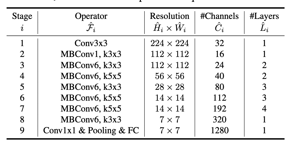
Figure 3: EfficientNet-B0 baseline architecture [ 4 ]
From the B0 architecture, we can derive scaled architectures labelled B1-B7 by:
Fix \(\phi=1\) and assume two times more resources are available (see Equation 1), and do a small grid search to find \(\alpha, \beta, \gamma\), which were \(\alpha=1.2, \beta=1.1, \gamma=1.15\) (depth, width, resolution, respectively), which give roughly 1.92 according to Equation 1.
Scale up the B0 architecture approximately using Equation 1 with the constants described in Step 1 by increasing \(\phi\) (and round where appropriate). Dropout is increased roughly linearly as the architectures grow from B0 (0.2) to B7 (0.5).
Table 1 shows the flops, multipliers and dropout rate for each dimension.
Name |
FLOPs |
Depth Mult. |
Width Multi. |
Resolution |
Dropout Rate |
|---|---|---|---|---|---|
efficientnet-b0 |
0.39B |
1.0 |
1.0 |
224 |
0.2 |
efficientnet-b1 |
0.70B |
1.1 |
1.0 |
240 |
0.2 |
efficientnet-b2 |
1.0B |
1.2 |
1.1 |
260 |
0.3 |
efficientnet-b3 |
1.8B |
1.4 |
1.2 |
300 |
0.3 |
efficientnet-b4 |
4.2B |
1.8 |
1.4 |
380 |
0.4 |
efficientnet-b5 |
9.9B |
2.2 |
1.6 |
456 |
0.4 |
efficientnet-b6 |
19B |
2.6 |
1.8 |
528 |
0.5 |
efficientnet-b7 |
47B |
3.1 |
2.0 |
600 |
0.5 |
For example, starting with B0, we have 0.39B FLOPs, going to B4 we have 4.2B flops, which yields \(\phi = 4.2 / 0.39 \approx 3.28\). This translates to scaling close to this value along the three dimensions with \(\alpha^{3.22} = 1.2^{3.22} \approx 1.8\), \(\beta^{3.53}=1.1^{3.53}\approx 1.4\), and \(\gamma^{3.78} = (1.15)^{3.78} \approx \frac{380}{224}\). We're not going for precision here, we just want a rough guideline of how to scale up the architecture. The nice thing about having this guideline is that we can create bigger ConvNets without having to do any additional architecture search.
1.4 Noisy Student
Noisy Student [5] is a semi-supervised approach to training a model that is useful even when you have abundant labelled data. This work is in the context of images where they show its efficacy on ImageNet and related benchmarks. The setup requires both labelled data and unlabelled data with a relatively simple algorithm (with some subtlety) and the following steps:
Train teacher model \(M^t\) with labelled images using a standard cross entropy loss.
Use the \(M^t\) (current teacher) to generate pseudo labels for the unlabelled data (filter and balance dataset as required)
Learn a student model \(M^{t+1}\) with equal or larger capacity on the labelled and unlabelled data with added noise.
Increment \(t\) (make the current student the new teacher) and repeat steps 2-3 as needed.
A few unintuitive points emphasized in bold. First, the student model uses an equal or larger model. This is different from other student/teacher paradigms where one is trying to distill the model knowledge into a smaller model. Here we're not trying to distill, we're trying to boost performance so we want a bigger model so it can learn from the bigger combined dataset. This seems to have a increase of 0.5-1.5% in top-1 ImageNet accuracy in their ablation study.
Second, the noise is implemented as randomized data augmentation plus dropout and stochastic depth. The added noise on the student seems to be around another 0.5% in top-1 ImageNet accuracy. Seems like a reasonable modification given that you typically want both of these things when training these types of networks.
Third, the iteration in step 4 also seemed important. Going from one iteration to three improved performance by 0.8% in top-1 ImageNet accuracy. It's not obvious to me that the performance would improve by iterating here but since the number of iterations is small, I can believe that it's possible.
Lastly, they discuss that they filter out pseudo labels that have low confidence by the teacher model, and then rebalance the unlabelled classes so the distribution is not so off (by repeating images). This also seems to improve performance a bit more modestly at 0-0.3% depending on the model.
The summary of the overall Noisy Student results are shown in Figure 4 where they conducted most of their experiments on EfficientNet. This figure only shows the non-iterative training (their headline result is within the iterative training). You can see that the Noisy Student dominates the vanilla EfficientNet results at the same number of model parameters and achieves SOTA (at the time of the paper). Note that the Noisy Student does have access to more unlabelled data than the EfficientNet, so perhaps it's not so surprising that it does better. In the context of this post, there are many versions of EfficientNet with Noisy Student training that are available for use as a pre-trained model.
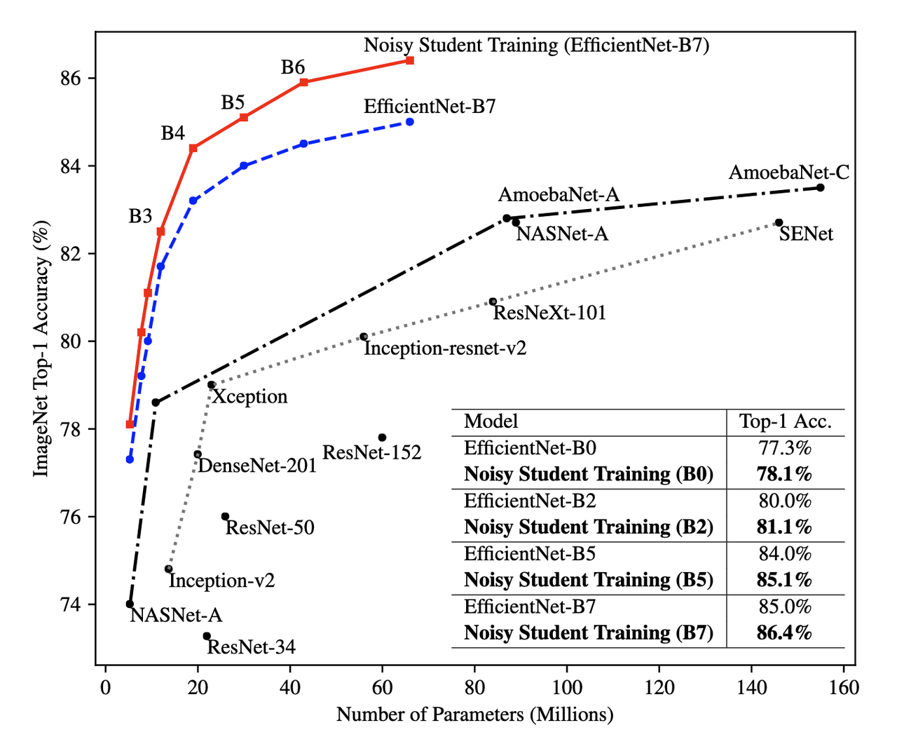
Figure 4: Noisy Student training shows significant improvement over all model sizes. [ 5 ]
2 SIIM-ISIC Melanoma Classification 2020 Competition
The Society for Imaging and Informatics in Medicine (SIIM) and the International Skin Imaging Collaboration (ISIC) melanoma classification competition [0] aims to classify a given skin lesion image and accompanying patient metadata as melanoma (or not). Melanoma is a type of skin cancer that is responsible for over 75% of skin cancer deaths. The ISIC has been putting on various computer vision challenges related to dermatology since 2016. Notably, past competitions have labelled image skin lesion data (and sometimes patient metadata) but with different labels that have partial overlap with the 2020 competition. More than 3300 teams participated in the competition with the winning solution [1] being the topic of this post.
The dataset consists of 33k training data points with only 1.76% positive samples (i.e., melanoma). Each datum contains a JPEG image of varying sizes (or a standardized 1024x1024 TFRecord) of a skin lesion along with patient data, which includes:
patient id
sex
approximate age
location of image site
detailed diagnosis (training only)
benign or malignant (training only, label to predict)
binarized version of target
Additionally, there were "external" data that one could use from previous years of the competition that had similar skin lesion images with slightly different tasks (e.g. image segmentation, classification with different labels etc.). This additional data made a combined dataset of roughly 60k images that one could possibly use.
The competition in 2020 was hosted on Kaggle which contained a leader board of all submissions. Each team submitted a blind prediction on the given test set and the leader board measured its performance using AUC. The leader board showed a public view on all submissions which showed the AUC score based on 30% of the test set. The remaining 70% of the testset remained hidden on the private leader board until the end of the competition and was used to evaluate the final result.
Table 2 shows several select submissions including the top 3 on the public and private leader boards. Interestingly, the top 3 winners on the private data all ranked relatively low, including the top submission which ranked all the way down at 881! Impressively, the top public score had a whopping 0.9931 AUC but only ended up at rank 275 in the final private ranking. The number of submissions is also interesting. Clearly, overfitting on the public test set was common as the top 3 winners all having relatively low number of submissions compared to others. The other obvious thing is that the scores are so close together that luck definitely played a role in the final ranking among the top submissions.
Private Rank |
Private Score |
Public Rank |
Public Score |
Submissions |
|---|---|---|---|---|
1 |
0.9490 |
881 |
0.9586 |
116 |
2 |
0.9485 |
57 |
0.9679 |
61 |
3 |
0.9484 |
265 |
0.9654 |
118 |
27 |
0.9441 |
2 |
0.9926 |
402 |
100 |
0.9414 |
329 |
0.9648 |
121 |
275 |
0.9379 |
1 |
0.9931 |
276 |
395 |
0.9357 |
3 |
0.9767 |
245 |
500 |
0.9336 |
241 |
0.9656 |
227 |
3 Winning Solution
The winning solution [1] to the SIIM-ISIC 2020 Competition used a variety of techniques that led to their outperformance. This section discusses some of those techniques.
3.1 Dataset Creation and Data Preprocessing
The winning solution used a preprocessed dataset that one of his colleagues created [6]. This dataset was in fact used by many of the competing teams and arguably one of the most critical pieces of work (something that a huge amount of time is spent on in real world problems).
The first step in preprocessing was center cropping and resizing the images. Many of the JPEG images were really large and had different dimensions (e.g., 1053x1872, 4000x6000, etc.) totalling 32GB. After reducing them down to various standard sizes (e.g. 512x512, 768x768, 1024x1024) they were much more manageable to use, for example the 512x512 dataset was about 3GB for 2020 data.
Next, the preprocessed dataset also contained a "triple" stratified 5-fold validation dataset:
Separate Patients: This stratification was to ensure that the same patient was not in both the train and validation set. This can happen when you have two skin lesion images from the same person, which is undesirable because the resulting diagnosis is likely highly correlated in these situations.
Positive Class: This stratification was to ensure that the positive classes were distributed correctly across each fold. Due to the highly imbalanced problem of only having 1.76% positive classes, ensuring an even balance across folds was very important.
Patient Representation: Some patients had only a few images while others had many. To have balanced folds, this stratification was to ensure that you have good representation of each across each fold as well.
Lastly, although the external data had a lot of additional images, many of them were in fact duplicates that should be removed. But this is harder than it looks because the images were not exact matches, for example they could be scaled and rotated, thus you cannot just compare the raw pixels. To have a clean validation set, you want to make sure you have a truly independent train and validation set. To solve this problem, the preprocessing in [6] used a pre-trained (EfficientNet) CNN to generate embeddings of each image, and then removed near duplicates (with manual inspection). Hundreds of duplicates were removed, making a much cleaner validation set.
3.2 Validation Strategy
The first place solution noted that one of the keys to winning was having a robust validation strategy, which was particularly important in this competition [6] (as well in the real world). As noted above, the original dataset had only a 1.76% positive rate over 33k training samples. That translates to around 580 positive samples, and barely over 100 samples when doing for a 5-fold cross validation. This naturally would lead to an unstable AUC (or pretty much any other metric you're going to use).
Beyond the training data provided, the test data that could be evaluated via the public leader board had only about 10k samples, 30% of which was used to evaluate AUC on the public leader board. If the distribution were similar in this test set, this would only leave about 50 or so positive test case samples. Thus, the public leader board evaluation was similarly unreliable and couldn't be used to robustly evaluate the model. This was clearly seen as the top 3 public leader ranks dropped significantly when evaluated on the private data set. The authors also mention that their cross validation scores (described below) were not correlated with the public leader board and that they basically ignored the leader board.
The winning solution instead utilized both the competition (2020) data and external data (2019) for training and validation. The 2019 data had 25k data points with a 17.85% positive rate, making it much more reliable when it was used for both training and validation.
The other key thing they did was to train on a multi-class problem instead of the binary target given by the competition. In the 2020 data, a detailed diagnosis column was given, while in the 2019 data, a higher-level multi-class label was given (vs. the binary label). As is typical in many problems, they leveraged some domain knowledge (using the descriptions from the competition) and mapped the 2020 detailed diagnosis to the 2019 labels shown in Figure 5. The main intuition of using a multi-class target is that it gives more information to the target when the lesion is benign (not cancerous).
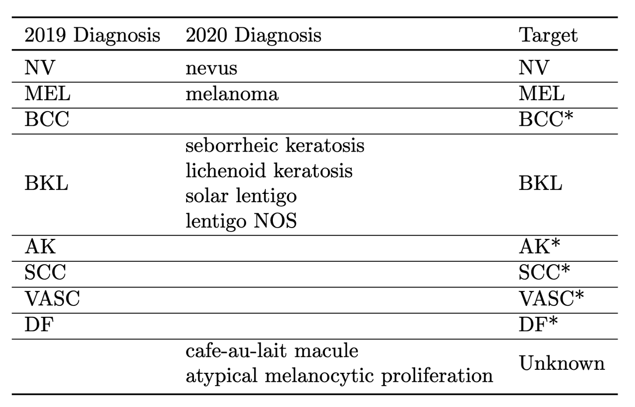
Figure 5: Mapping from diagnosis to targets [ 1 ]
When evaluating the model the primary evaluation metric is the binary classification AUC of the combined 2019 and 2020 cross validation folds (the multi-class problem can easily be mapped back to a binary one). The cross validation AUC of the 2020 dataset was used as a secondary metric.
3.3 Architecture
The solution consisted of an ensemble of eighteen fine-tuned pre-trained ConvNets shown in Figure 6 that were combined using a simple average of ranks. Notice that the first 16 models are EfficientNet variants from B3 all the way to B7, while the last two are SE-ResNext101 and Nest101. For the EfficientNet variants, besides the model size, the models vary by the image input sizes (384, 448, 512, 576, 640, 768, 896) deriving from the next largest source image in the above described dataset (512, 768, 1024). The different models plus image sizes is an important source of diversity in the ensemble. Unfortunately, the authors didn't describe how they selected their ensemble except to say that diversity was important. Interestingly, the authors state [6] that the CNN backbone isn't all that important and they mostly just picked an off-the-shelf state-of-the-art model architecture (EfficientNet) where pre-trained models and code are readily available.
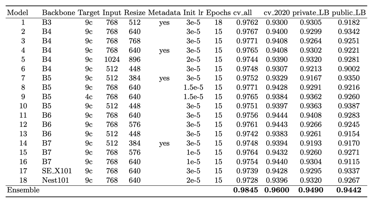
Figure 6: Model configurations for winning solution ensemble and their AUC scores [ 1 ]
The ensembles also varied based on their use of metadata with tuned learning rates and epochs for each configuration. The authors mention [6] that the metadata didn't seem to help much with their best single model not using metadata. They hypothesize that most of the useful information is already included in the image. However, they think it was useful in providing diversity in the ensemble (again being one of the most important parts of ensembling). Additionally, one of the models only used a reduced target with 4 classes (collapsing the "*" labels in Figure 5).
Another interesting part is how they incorporated the metadata with the images. Figure 7 shows the architecture with metadata. The metadata network is relatively simple with two fully connected layers whose output is concatenated with the CNN before the last classification layer. They use a pretty standard architecture with BatchNorm and dropout, but they do use the Swish activation.
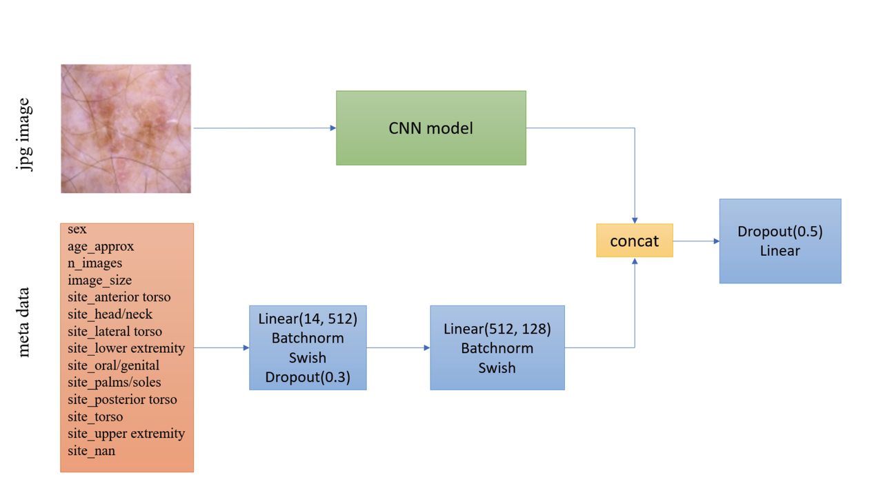
Figure 7: Model architecture including metadata [ 1 ]
Lastly, I noticed a trick that I had not seen before in the last linear classification layer. They use five copies of the linear layer (shared params) each with a different dropout layer, which then are averaged together to generate the final output shown in Listing 5. My guess to its purpose is that it is trying to remove the randomness of dropout, which may be important since it's so high at a 0.5 dropout rate.
for dropout in enumerate(self.dropouts):
    if i == 0:
        out = self.myfc(dropout(x))
    else:
        out += self.myfc(dropout(x))
out /= len(self.dropouts)
Listing 5: Last layer of Winning Solution ( source )
Ensembles Selection Ideas from Another Solution
In addition to the explanation of [1] in the YouTube video [6], one of their colleagues from Nvidia also presented their solution, which also got a gold medal coming in 11th. Their solution was more "brute force" (in their own words) building hundreds of models and relied on some strategies to whittle it down to their final ensemble. Two interesting ideas for ensemble selection came out in the explanation of their solution:
"Correlation Matrix Divergence": The idea is you want to filter out models that are overfitting on the training data. So for each model, compute the correlation matrix over all classes on the training set, then do the same on the test set. Then you subtract the two and look for values in the difference that are large. The intuition is that if there is a big divergence then the model may not be generalizing well to the test set for various reasons from overfitting to bugs. So the team used this as a filter to remove models that were highly "divergent".
"Adversarial Validation Importances": Build a model that takes as input all the predictions from the candidate set of models to predict whether an image is in the train or test set. If the set of models can easily detect the test set, then that means you are picking up on a signal that is biased towards one or the other. Using (I assume) feature importances, you can find which models are contributing to this signal and remove it. Similar to the other method, you want to make it so the models in your ensemble cannot distinguish between train and test to ensure they are going to generalize well.
For both of these methods you will need to use your judgement on which threshold to set to drop models. The authors just said they used their best guess and didn't have a methodical way.
3.4 Augmentation
Data augmentation is a common method to improve vision models and many libraries are readily available for standard transformations. The winning solution used the albumentations library that has a rich variety of image transformations that are performant and easily accessible.
The authors used a whole host of transformations where you can see the code here. I'll mention a few interesting points I found:
The last transformation always resizes the image back to the target size.
They use the
compose()function to apply all transformations to each image, however (in most cases) each transformation will have some probability of activating or not.They'll also have some
OneOfchoices in there for blurring (Motion, Median, Gaussian, GaussNoise blurring) and distortion (OpticalDistortion, GridDistortion, ElasticTransform).Some of the transforms require more careful setting of parameters that depend on the domain. For example the
Cutouttransform, which blanks out a square region of the image, requires a bit more careful thinking to ensure that the region isn't too large. In this case, they used a single 37.5% of image sized square to cutout with 70% probability.The transformations are only on the training set. The validation set transforms are only used to preprocess the image for the model by doing a resize and normalization.
3.5 Prediction
On the prediction side there were a couple tricks that I thought are worth mentioning:
Fold Averaging: The best model from each of the 5 validation folds is saved based on the validation dataset AUC. This means for every ensemble model (total 18), we have 5 trained models. The prediction for a single model is generated by averaging the 5 probabilities. That is, for each of the 5 trained models (identical configurations but different folds), compute the mean across the 5 models for each softmax output separately.
-
Orientation Averaging: Due to the nature of the images, the solution (for each of the above fold models) averaged 8 different predictions per model, where each prediction was given a different orientation of the input image. This means for each model configuration you have 5 x 8 predictions, which are averaged by their probabilities.
The different orientations are: original, horizontal flip, vertical flip, horizontal & vertical flip, diagonal "flip" (transpose), diagonal & horizontal flip, diagonal & vertical flip, diagonal & horizontal & vertical flip. For skin lesions the orientation probably doesn't matter at all, so computing the average over many different orientations probably smooths out any quirks the models has with a particular orientation. Intuitively, I would guess this increases the robustness of the model's prediction. See the source for the details on both of these tricks.
Ensemble Construction: From each of the above 18 model configurations after averaging you have a single column of probabilities corresponding to the test set data. To generate the final prediction, we do a "rank average": convert all the probabilities in a column to ranks, normalize those relative ranks to between 0 and 1 (as a percentage), and finally compute a simple mean between all of the columns. This is probably more robust than computing a simple probability average because it does not overweight confident models that might output very high (or low) probability values.
3.6 Training Details
Here are the details for the training:
Epochs: 15 for most models. I'm going to guess (because they didn't specify) that they picked a large enough number so that the AUC didn't continue to increase but also balanced with a manageable run-time. Since they save the best model in the fold (according to the validation AUC), as long as this number is big enough you're only losing run-time.
Batch size: 64 for all models. They mentioned (I believe) that it was easier to just keep it all the same for each model than try to tune it, presumably because batch size wasn't expected to make much of a difference.
Learning rate/schedule: Ranged from \(1e-5\) to \(3e-5\) with a cosine cycle, where the learning rate is tuned for each model (recall this is fine-tuning a pre-trained ImageNet model). There is also a single warm-up epoch at the beginning which is one tenth of the initial learning rate.
Optimizer: Adam. Stated that using a standard strong optimizer was good enough.
Hardware: Trained on V100 GPUs in mixed precision mode with up to 8 GPUs used in a data parallel (batch split across GPUs) manner.
4 Experiments
The experiments I conducted consisted of a bunch of ablation tests against a baseline configuration because I was curious about the importance of each of the decisions in the winning solutions. Due to only having access to my local RTX 3090 (and not wanting to spend more on cloud compute), I ran it versus a smaller baseline than the models used in the original solution. On the baseline setup, running 3 folds (vs. 5) took roughly one full day (which could have been faster, see my notes on improving run-time below). Notably, I didn't try many bigger models because I didn't want to spend time waiting around for them to finish.
You can see the script I used to run it here, which just used the existing training script (plus a few new arguments to test some of the techniques). The baseline setup was as follows (parentheses denoting the original setup):
3 fold cross training (vs. 5 folds), 15 epochs per fold
Use external data from the preconstructed dataset but no patient level data (i.e., only images)
Image size 384 (vs. 448-896 resolution)
Architecture: EfficientNet B3 (vs. B4-B7, SE-ResNext101 and ResNest101)
Cosine cycle with warm-up epoch
Batch size: 48 (vs. 64) to fit on my GPU memory
LR: 3e-5
Relative to this baseline setup, I'll discuss the things that seemed to be make a significant difference in the validation scores and those that didn't.
4.1 Changes That Showed Improvement
Figure 8 shows the experiments that appears to have improved performance beyond
just randomness. The figure shows (a) the mean best AUC across the three
folds measured on the validation set which includes external data (AUC_mean),
and (b) the similarly calculated AUC for the validation set with just the 2020
competition data (AUC_20_mean). Error bars indicate the standard
deviation computed across the best AUC score across the three folds. Starting
left to right, the changes from the baseline were:
baseline: Baseline setup described above.
no-pretraining: Did not used a pre-trained B3 model.
no-augmentation: Removed data augmentation transforms.
no-external-data: A run that only utilized training data from the 2020 competition data set (no previous years).
warmup: Remove the first warmup epoch which starts at a tenth of the initial learning rate and gradually grows to the target LR by the end of the epoch.
no-cosine: Did not use cosine learning schedule (which was implemented as one cycle across all epochs).
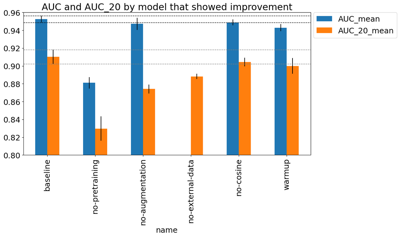
Figure 8: Experiments that showed improvement
As you can see, there are only a few things that are obviously beneficial particularly relating to the data. The biggest gain appears to be due to pre-training, which is around an 0.08 AUC gap from the baseline. This makes sense since we only have around 60K data points, so pre-training (even on an unrelated ImageNet dataset) would be useful. The other big drop seems to be whether or not we're using data augmentation. Although the AUC metric seems like it might be only a small drop, the AUC_20 shows quite a large one, indicating that this plays a significant role in the performance. Another important data related change was the use of external data. The AUC metric is not reported because the default computation from the script was not comparable (and I didn't feel like hacking it to make it comparable). Instead, we can see the AUC_20 metric which shows about a 0.03 AUC gap. These results really show the value of adding more data (in whatever form) leads to the most durable boosts to performance.
The two other more minor improvements come from the learning rate schedules with a warmup epoch and a cosine scheduling of learning rates. The warmup seemed the most significant with 0.02 AUC difference with the cosine scheduling showing very minor improvement with 0.01 AUC (possible that it's not significant). Although it could be noise, they seem like relatively harmless improvements, which are highly likely to give a small boost to performance.
4.2 Changes That Did Not Showed Improvement
Similar to the changes that showed improvement, I ran a bunch of other experiments shown in Figure 9 with the same metrics. For the most part, they did not show significant improvement over the baseline. Starting from left to right in Figure 9, the changes were:
baseline: Baseline setup described above.
+noisy-student: Use a pre-trained B3 model with Noisy Student training.
effnet_b2: Use EfficientNet B2 model instead of B3.
lr={1.5e-5, 2e-5}: Use a learning rate of 1.5e-5, 2e-5 (vs. 3e-5).
+metadata: Utilize patient (non-image) metadata.
dropout-layers={1, 3}: Utilize 1, 3 parallel dropout layers (vs 5) as described above in the Architecture section.
img_size=448: Utilize image size of 448 (vs. 384).
binary_labels: Utilize binary labels in training (as the competition expects) instead of 9 classes.
tensorflow_impl: Utilize a tensorflow implementation of the pre-trained model.
amp: Utilize Automated Mixed Precision (AMP) in PyTorch.
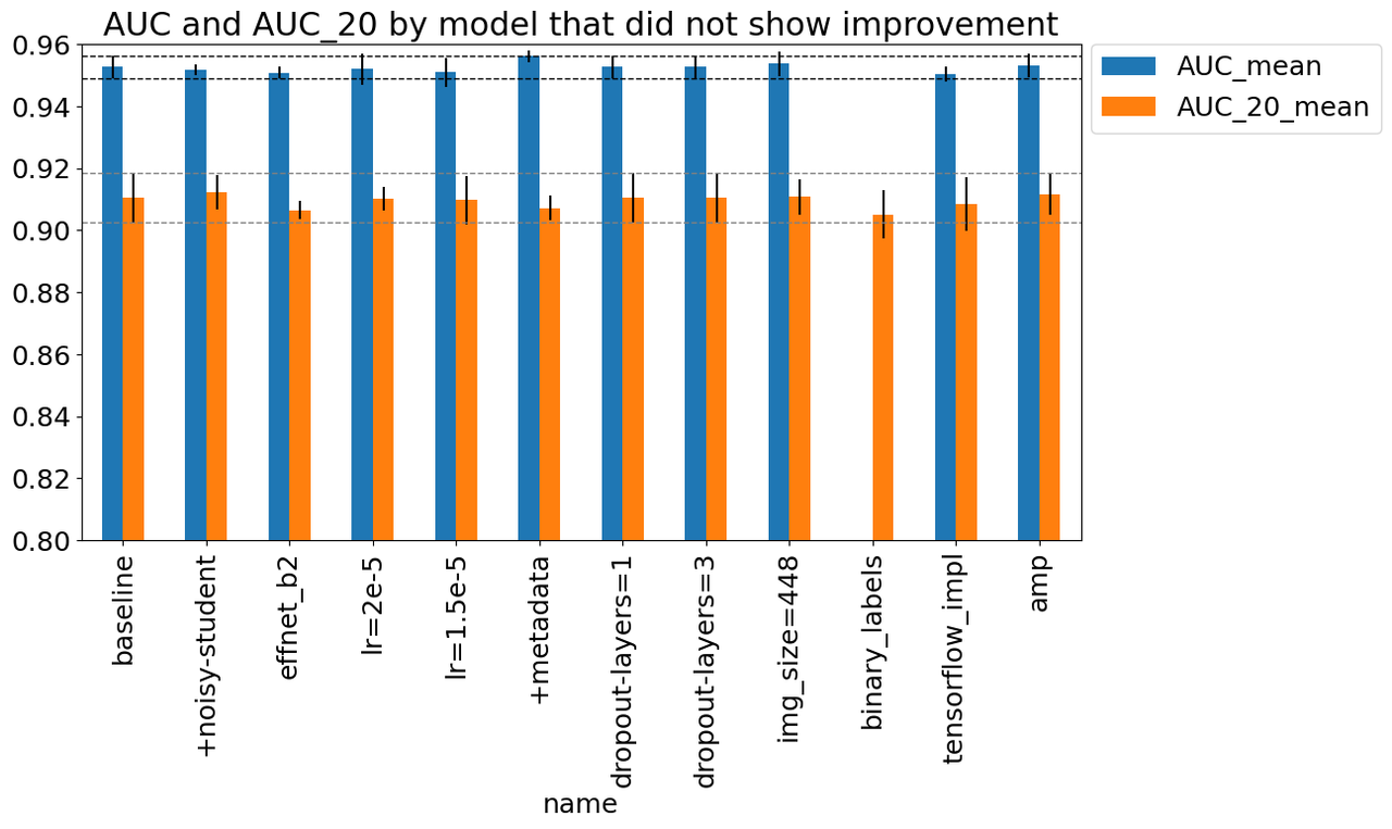
Figure 9: Experiments that did not showed improvement
I'll just comment on a few things that were surprising:
"Fancy" things didn't seem to be that important. For example, Noisy Student or changing architecture to B2 didn't seem to do much. Similarly the dropout layers didn't change things much.
Implementation details didn't seem to make a big difference like the Tensorflow implementation or using AMP.
Not very sensitive to many hyperparameters like learning rate and image size. Although I suspect it could be because we're fine-tuning vs. doing direct training. The learning rate is so small (and we have a lot of epochs) so it may not make a big difference.
One thing I did find surprising was that the binary labels didn't didn't make that much of a difference. Intuitively, it feels like better categories would encourage better learning but even if it did, it looks like it wasn't that significant. It could be because the different classes were all distinguishing the negative labels, never the difference between positives and negative. Similar to the previous section, this experiment only had an AUC_20 measure since the problem formulation was different.
One of things that was borderline useful was the use of metadata, which I included in this section instead of the one above. The paper states that metadata didn't in general do much but was useful to make more diverse models. In my experiments, it's not significant but it's possible it does help, perhaps especially in smaller models/image sizes like B3/384x384. It's hard to draw conclusions though.
In general, as is the case in many of these situations, there are not many silver bullets. Most things do not significantly improve the performance of the problem in a real world scenario. Or at least they're not "first order" improvements that you would try on a first pass of a problem. If you're optimizing for a 0.1% improvement (e.g. AdWords) then you might want to spend more time with these "second order" improvements to hyper-optimize things. Although these experiments are not extensive, they probably point directionally to what you should care about: data and maybe better learning schedules.
4.3 Training Time
For most of my experiments, a typical run would take about 27 hours (about 37 mins / epoch) for the baseline setup. This seemed kind of unreasonably long for a small B3 setup, but I mostly ignored it because I was just queueing the jobs up and coming back to next day to see what happened. I even noticed that the GPU utilization was low but ignored it thinking it was a weird artifact of my training setup. At one point late in my experiments, I started playing around with AMP and PyTorch 2.0 compilation but didn't see a significant change in run-time.
Only after I had the idea to run the data augmentation experiment did I realize
my issue: the data augmentation transforms were bottlenecking my batches! I
had been using a single thread for the DataLoader (which I did to avoid
an error initially, see notes below), which caused most of the run-time to be on my CPU. After
increasing the number of workers to 6 (the number of cores on my CPU), I got
the run-time down to less than 10 minutes per epoch with relatively high GPU
utilization.
Most of my previous explorations have been on relatively smaller models (partly because I had a small 8GB 1070 up until last year) so I didn't have to think too much about run-time. But now that I'm running bigger jobs, savings 3-4x in run-time is pretty significant even though I typically leave it running for 24 hours between experiments (because I only work on these projects in the evening). I think I'll be looking more into the basics of optimizing run-time in the near future.
5 Miscellaneous Notes
Here are a bunch of of random thoughts I had while doing this project.
W&B: This is the first project that I used Weights and Biases extensively, and it's really good! It was easy to start logging things using Github CoPilot (it auto-filled my wandb.log() statement) and getting them to show up in a pretty dashboard (including system performance metrics). It's really nice not to have to think about collecting data from experiments. Analysis of the results was equally easy. I had to do something more custom (because I didn't record the best AUC from each fold), and it was really easy to use a notebook to download the raw data via the W&B API and compute the metrics I needed. It made it so I didn't have to waste a lot of time doing this boring work. The one thing to remember for future projects is to tag my runs better so it makes it easier to view in the W&B GUI instead of clicking in to see what the command line arguments were.
Github CoPilot: I have recently started to use the Github CoPilot Chat functionality in VSCode. I initially didn't know it was there! So it's basically ChatGPT but I suppose with a model tuned more to code (and a different default prompt). It also automatically takes the context within range of your cursor so it can easily explain things better than just using vanilla ChatGPT. In addition to the auto-complete, I found it extremely useful because it was usually faster and more helpful than trying to lookup the documentation on the web myself. I will say there was one or two instances where it was not giving me the answer I wanted, and I had a hunch that an even better solution would be for it to answer AND point to the original documentation (using Retrieval Augmented Generation or something like that). Maybe they'll add that someday. In any case, even though I only use it for side projects, it's 100% worth the $10/month that I pay.
Plotting with CoPilot: CoPilot makes Python plotting so easy! I'm not sure about you but previously I always looked up canned examples of how to plot in Matplotlib/Pandas, which always had some unintuitive part that was confusing, never mind details like a legend or grouped bar charts were always very esoteric or complicated. Now CoPilot will get my chart 95% of the way there (with correct syntax) and then it's easy for me to modify it. LLM's for the win!
I had a minor Docker shared memory issue when I increased the number of workers in the
DataLoader. The training script would die with a not enough shared memory error. And while I gave it a generous 1 GB of shared memory, it turns out it was not enough. In Linux (POSIX standard),/dev/shmis a shared memory space with a filesystem-like interface that uses RAM to help facilitate interprocess communication. Since theDataLoaderuses multiple processes it used up a surprisingly large amount of space to prepare images (at least that's what it looked like). The fix was easy: increase the space to 8GB, which cleared up my problem. You can see my Docker run script and the other scripts that I used to set up my environment in this repo.
6 Conclusion
It never ceases to amaze me how much there is to learn from diving deep into a subject. While the original write-up to the Kaggle solution was only a few pages long (single column), the YouTube video and the code repo added a lot more layers, and digging into some of the ML techniques added even more. It was a fun (and educational) exercise to understand what choices were actually important. It was also very useful getting schooled on the importance of optimizing long running jobs on the GPU. And despite this longish write-up, there's still so much more that I still want to dig into (e.g. PyTorch run-time optimizations) but this post has already become longer than I expected (as usual). That's it for now, thanks for reading!
7 References
[0] SIIM-ISIC Melanoma Classification Kaggle Competition
[1] Qishen Ha, Bo Liu, Fuxu Liu, "Identifying Melanoma Images using EfficientNet Ensemble: Winning Solution to the SIIM-ISIC Melanoma Classification Challenge", https://arxiv.org/abs/2010.05351
[2] Sandler et al. "MobileNetV2: Inverted Residuals and Linear Bottlenecks", CVPR 2018, https://arxiv.org/abs/1801.04381
[3] Hu et al. "Squeeze-and-Excitation Networks", CVPR 2018, https://arxiv.org/abs/1801.04381
[4] Mingxing Tan, Quoc V. Le, "EfficientNet: Rethinking Model Scaling for Convolutional Neural Networks", https://arxiv.org/abs/1905.11946
[5] Xie et al. "Self-training with Noisy Student improves ImageNet classification", https://arxiv.org/abs/1911.04252
[6] Nvidia Developer, "How to Build a World-Class ML Model for Melanoma Detection", https://www.youtube.com/watch?v=L1QKTPb6V_I