Normalizing Flows with Real NVP
This post has been a long time coming. I originally started working on it several posts back but hit a roadblock in the implementation and then got distracted with some other ideas, which took me down various rabbit holes (here, here, and here). It feels good to finally get back on track to some core ML topics. The other nice thing about not being an academic researcher (not that I'm really researching anything here) is that there is no pressure to do anything! If it's just for fun, you can take your time with a topic, veer off track, and the come back to it later. It's nice having the freedom to do what you want (this applies to more than just learning about ML too)!
This post is going to talk about a class of deep probabilistic generative models called normalizing flows. Alongside Variational Autoencoders and autoregressive models 1 (e.g. Pixel CNN and Autoregressive autoencoders), normalizing flows have been one of the big ideas in deep probabilistic generative models (I don't count GANs because they are not quite probabilistic). Specifically, I'll be presenting one of the earlier normalizing flow techniques named Real NVP (circa 2016). The formulation is simple but surprisingly effective, which makes it a good candidate to understand more about normalizing flows. As usual, I'll go over some background, the method, an implementation (with commentary on the details), and some experimental results. Let's get into the flow!
Table of Contents
1 Motivation
Given a distribution \(p_X(x)\), deep generative models use neural networks to model \(X\), usually by minimizing some quantity related to the negative log-likelihood (NLL): \(-\log p_X(x)\). Assuming we have identical, independently distributed (IID) samples \(x \in X\), we are aiming for a loss that is related to:
There are multiple ways to build a deep generative model but a common way is to use is a latent variable model, where we partition the variables into two sets: observed variables (\(x\)) and latent (or hidden) variables (\(z\)). We only ever observe \(x\) and only use the latent \(z\) variables because they make the problem more tractable. We can sample from this latent variable model by having three things:
Some prior \(p_Z(z)\) (usually Gaussian) on the latent variables;
Some high capacity neural network \(g(z; \theta)\) (a deterministic function) with input \(z\) and model parameters \(\theta\);
A conditional output distribution \(p_{X|Z}(x|g_(z; \theta))\) that use the outputs of the neural network to model the data distribution \(X\) (via an appropriate loss function).
By sampling \(z\) from our prior and passing it through our neural network to define our conditional output distribution \(p_{X|Z}\) for the given \(z\), we can then use it to (often explicitly) sample our \(X\). In these cases, sampling is usually relatively straight forward but training on the other hand is not. Let's see why.
We wish to minimize Equation 1 (our loss function) but we only have our conditional distribution \(p_{X|Z}\). We can get most of the way there by using our prior \(p_Z\). From Equation 1:
There are a couple of issues here. First, we have this summation inside the logarithm, that's usually a tough thing to optimize. Perhaps the more important issue though is that we have to draw \(K\) samples from \(Z\) for every \(X\). If we use any reasonable number of latent variables, we immediately hit the curse of dimensionality for the number of samples we need.
Variational autoencoders are a clever way around this by approximating the posterior with another deep net that simultaneously trains with our latent variable model. Using the expected lower bound objective (ELBO), we can indirectly optimize (an upper bound of) \(-\log p_X(x)\). See my post on VAEs for more details.
This is great but can we define a deep generative model that does this more directly? What if we could directly optimize \(p_X(x)\) but still have the nice properties of a latent variable model? What special setup of the problem do we need to maintain to allow for this? Keep on reading to find out more!
2 Background
The first two concepts we need are the Inverse Transform Sampling and Probability Integral Transform. Inverse transform sampling is idea that given a random variable \(X\) (under some mild assumptions) with CDF \(F_X\), we can sample from \(X\) starting from a standard uniform distribution \(U\). This can be easily seen by sampling \(U\) and using the inverse CDF \(F^{-1}_X\) to generate a random sample from \(X\). The probability integral transform is the opposite operation: given a way to sample \(X\) (and its associated CDF), we can generate a sample from a standard uniform distribution \(U\) as \(u=F_X(x)\). See the box below for more details.
Using these two ideas (and its extension to multiple variables), there exists a deterministic transformation (recall CDFs are deterministic and invertible functions) to go from any distribution \(X\) to any distribution \(Y\). This can be achieved by transforming from \(X\) to a standard uniform distribution \(U\) (probability integral transform) then going from \(U\) to \(Y\) (inverse transform sampling). For our purposes, we don't actually care to explicitly specify the CDFs but rather just understand that this transformation from samples of \(X\) to \(Y\) exists via a deterministic function. Notice that this deterministic function is bijective (or invertible) because the CDFs (and inverse CDFs) are monotone functions.
Inverse Transform Sampling
Inverse transform sampling is a method for sampling from any distribution given its cumulative distribution function (CDF), \(F(x)\). For a given distribution with CDF \(F(x)\), it works as such:
Sample a value, \(u\), between \([0,1]\) from a uniform distribution.
Define the inverse of the CDF as \(F^{-1}(u)\) (the domain is a probability value between \([0,1]\)).
\(F^{-1}(u)\) is a sample from your target distribution.
Of course, this method has no claims on being efficient. For example, on continuous distributions, we would need to be able to find the inverse of the CDF (or some close approximation), which is not at all trivial. Typically, there are more efficient ways to perform sampling on any particular distribution but this provides a theoretical way to sample from any distribution.
Proof
The proof of correctness is actually pretty simple. Let \(U\) be a uniform random variable on \([0,1]\), and \(F^{-1}\) as before, then we have:
Thus, we have shown that \(F^{-1}(U)\) has the distribution of our target random variable (since the CDF \(F(x)\) is the same).
It's important to note what we did: we took an easy to sample random variable \(U\), performed a deterministic transformation \(F^{-1}(U)\) and ended up with a random variable that was distributed according to our target distribution.
Example
As a simple example, we can try to generate an exponential distribution with CDF of \(F(x) = 1 - e^{-\lambda x}\) for \(x \geq 0\). The inverse is defined by \(x = F^{-1}(u) = -\frac{1}{\lambda}\log(1-y)\). Thus, we can sample from an exponential distribution just by iteratively evaluating this expression with a uniform randomly distributed number.
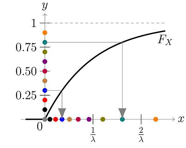
Figure 1: The \(y\) axis is our uniform random distribution and the \(x\) axis is our exponentially distributed number. You can see for each point on the \(y\) axis, we can map it to a point on the \(x\) axis. Even though \(y\) is distributed uniformly, their mapping is concentrated on values closer to \(0\) on the \(x\) axis, matching an exponential distribution (source: Wikipedia).
Extensions
Now instead of starting from a uniform distribution, what happens if we want to sample from another distribution, say a normal distribution? We just first apply the reverse of the inverse sampling transform called the Probability Integral Transform. So the steps would be:
Sample from a normal distribution.
Apply the probability integral transform using the CDF of a normal distribution to get a uniformly distributed sample.
Apply inverse transform sampling with the inverse CDF of the target distribution to get a sample from our target distribution.
What about extending to multiple dimensions? We can just break up the joint distribution into its conditional components and sample each sequentially to construct the overall sample:
In detail, first sample \(x_1\) using the method above, then \(x_2|x_1\), then \(x_3|x_2,x_1\), and so on. Of course, this implicitly means you would have the CDF of each of those distributions available, which practically might not be possible.
The next thing we need is to review is how to change variables of probability density functions. Given continuous n-dimensional random variable \(Z\) with joint density \(p_Z\) and a bijective (i.e. invertible) differentiable function \(g\), let \(X=g(Z)\), then \(p_X\) is defined by:
where \(det\big(\frac{\partial f(x)}{\partial x}\big)\) is the determinant of the Jacobian matrix. The determinant comes into play because we're changing variables of the probability density function in the CDF integral so the usual rules of change of variable for integrals apply.
We'll see later that using this change of variable formula with the (big) assumption of a bijective function, we can eschew the approximate posterior (or in the case of GANs the discriminator network) to train our deep generative model directly.
3 Normalizing Flows with Real NVP
The two big ideas from the previous section come together using this simplified logic:
There exists an invertible transform \(f: X \rightarrow Z\) to convert between any two probability densities (Inverse Transform Sampling and Probability Integral Transform); define a deep neural network to be this invertible function \(f\).
We can compute the (log-)likelihood of any variable \(X=f^{-1}(Z)\) (for invertible \(f\)) by just knowing the density of \(Z\) and the function \(f\) (i.e. not explicitly knowing the density of \(X\)) using Equation 5.
Thus, we can train a deep latent variable model directly using its log-likelihood as a loss function with simple latent variables \(Z\) (e.g Gaussians) and an invertible deep neural network (\(f\)) to model some unknown complex distribution \(X\) (e.g. images).
Notice the two things that we are doing that give normalizing flows [2] its name:
"Normalizing": The change of variable formula (Equation 5) gives us a normalized probability density.
"Flow": A series of invertible transforms that are composed together to make a more complex invertible transform.
Now the big assumption here is that you can build a deep neural network that is both invertible and can represent whatever complex transform you need. There are several methods to do this but we'll be looking at one of the earlier ones call Real-valued Non-Volume Preserving (Real NVP) transformations, which is surprisingly simple.
3.1 Training and Generation
As previously mentioned, normalizing flows greatly simplify the training process. No need for approximate posteriors (VAEs) or discriminator networks (GANs) to train -- just directly minimize the negative log likelihood. Let's take a closer look at that.
Assume we have training samples from a complex data distribution \(X\), a deep neural network \(z = f_\theta(x)\) parameterized by \(\theta\), and a prior \(p_Z(z)\) on latent variables \(Z\). From Equation 5, we can derive our log-likelihood function like so:
As in many of these deep generative models, if we assume a standard independent Gaussian priors for \(p_Z\), we can replace the first term in Equation 6 with the logarithm of the standard normal PDF:
Thus, our training is straight forward, just do a forward pass with training example \(x\) and do a backwards pass using the negative of Equation 7 as the negative log-likelihood loss function. The tricky part is defining a bijective deep generative model (described below) and computing the determinant of the Jacobian. It's not obvious how to design an expressive invertible deep neural network, and it's even less obvious how to compute its Jacobian determinant efficiently (recall the Jacobian could be very large). We'll cover both in the following subsections.
Generating samples is also quite straight forward because \(f_\theta\) is invertible. Starting from a randomly sample point from our prior distribution on \(Z\) (e.g. standard Gaussian), we can generate a sample easily by using the inverse of our deep net: \(x = f^{-1}_\theta(z)\). So a nice property of normalizing flows is that the training and generation of samples is fast (as opposed to autoregressive models where generation is very slow).
3.2 Coupling Layers
So the key question for normalizing flows is how can you define an invertible deep neural network? Real NVP uses a surprisingly simple block called an "affine coupling layer". The main idea is to define a transform whose Jacobian forms a triangular matrix resulting in a very simple and efficient determinant computation. Let's first define the transform.
The coupling layer is a simple scale and shift operation for some subset of the variables in the current layer, while the other half are used to compute the scale and shift. Given D dimensional input variables \(x\), \(y\) as the output of the block, and \(d < D\):
where \(s\) is for scale, \(t\) is for translation, and are functions from \(R^d \mapsto R^{D-d}\), and \(\odot\) is the element wise product. The reverse computation is just as simple by solving for \(x\) and noting that \(x_{1:d}=y_{1:d}\):
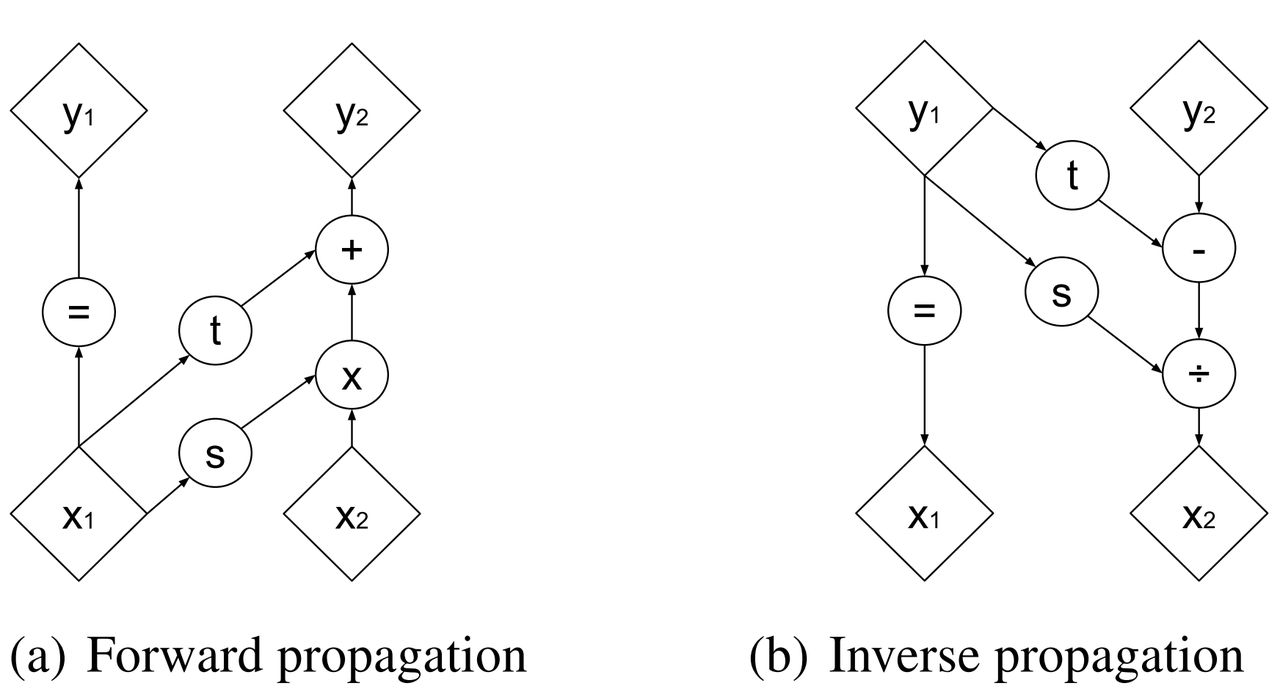
Figure 2: Forward and reverse computations of affine coupling layer [1]
Figure 2 from [1] that shows this visually. It's not at all obvious (at least to me) that this simple transform can represent the complex bijections that we want from our deep net. However, I'll point out two ideas. First, \(s(\cdot)\) and \(t(\cdot)\) can be arbitrarily deep networks with width greater than the input dimensions because they do not need to be inverted. This essentially lets the coupling block scale and shift (a subset of) the input \(x\) in complex ways. Second, we're going to be stacking a lot of these together. So while it seems like for a subset of the variables (\(x_{1:d}\)) we're not doing anything, in fact, we scale and shift every input variable multiple times. Still, there's no proof or guarantees in the paper that these transforms can represent every possible bijection but the empirical results are surprisingly good.
From our coupling layer in Equation 8, we can easily derive the Jacobian from Equation 6:
The main thing to notice is that it is triangular, which means the determinant is just the product of the diagonals. The first \(x_{1:d}\) variables are unchanged, so those entries in the Jacobian are just the identify function and zeros. The other \(x_{d+1:D}\) variables are scaled by \(exp(s(\cdot))\), so their gradient with respect to themselves is just a diagonal matrix of the scaling values, which form the other part of the diagonal. The other non-zero, non-diagonal part of the Jacobian can be ignored because it's never used. Putting this all together, the logarithm of the Jacobian determinant simplifies to:
which is just the sum of the scaling values (all the other diagonal values are \(\log (1) = 0\)).
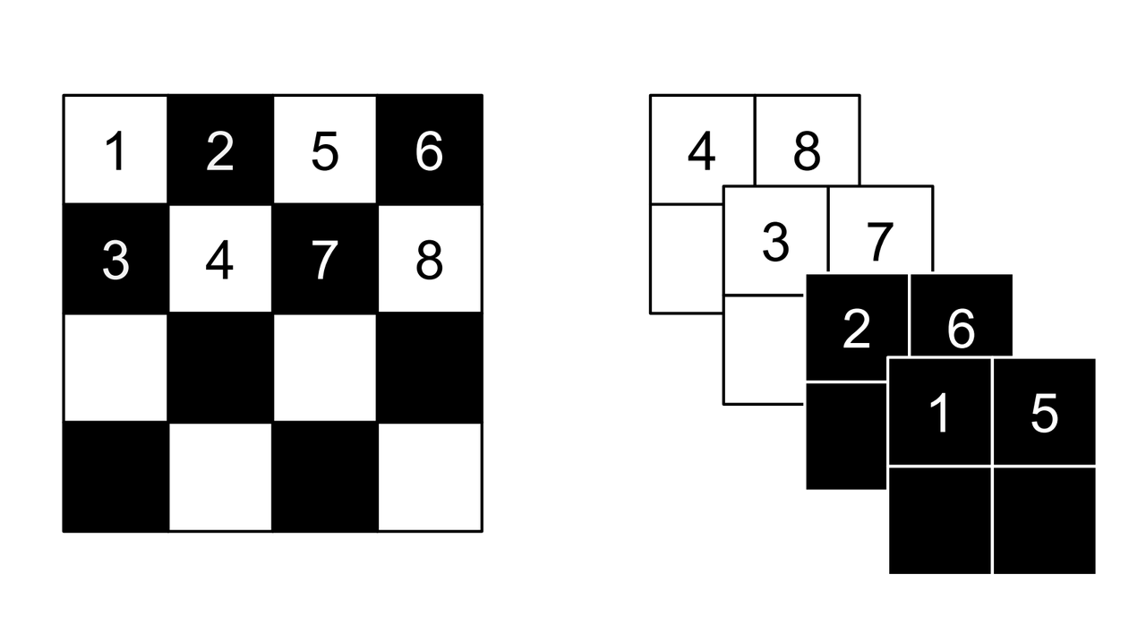
Figure 3: Masking schemes for coupling layers indicated by black and white: spatial checkerboard (left) and channel wise (right). Squeeze operation (right) indicated by numbers. [1]
Partitioning the variables is an important choice since you will want to make sure you have good "mixing" of dimensions. [1] proposes two schemes where \(d=\frac{D}{2}\). Figure 3 shows these two schemes with black and white squares. Spatial checkerboarding masking simply uses an alternating pattern to partition the variables, while channel-wise masking partitions the channels.
Although it may seem tedious to code up Equation 8, one can simply implement the partitioning schemes by providing a binary mask \(b\) (as shown in Figure 3) and use an element-wise product:
Finally, the choice of architecture for \(s(\cdot)\) and \(t(\cdot)\) functions is important. The paper uses Resnet blocks as a backbone to define these functions with additional normalization layers (see more details on these and other modifications I did below). But they do use a few interesting things here that I want to call out:
On the output of the \(s\) function, they use a tanh activation multiplied by a learned scale parameter. This is presumably to mitigate the effect of using exp(s) to scale the variables. Directly using the outputs of a neural network could cause big swings in \(s\) leading to blowing up \(exp(s)\).
To this point, they also add a small \(L_2\) regularization on \(s\) parameters of \(5\cdot 10^{-5}\).
On the output of the \(t\) function, they use an affine output since you want \(t\) to be able to shift positive or negative.
3.3 Stacking Coupling Layers
As mentioned before, coupling layers are only useful if we can stack them (otherwise half of the variables would be unchanged). By using alternating patterns of spatial checkerboarding and channel wise masking with multiple coupling layers, we can ensure that the deep net touches every input variable and that it has enough capacity to learn the necessary invertible transform. This is directly analogous to adding layers in a feed forward network (albeit with more complexity in the loss function).
The Jacobian determinant is straightforward to compute using the multi-variate product rule:
So in our loss function, we can simply add up all the Jacobian determinants of our stacked layers to compute that term.
Similarly, the inverse can be easily computed:
which basically is just computing the inverse of each layer in reverse order.
Data Preprocessing and Density Computation
A direct consequence of Equation 5-7 is that any preprocessing transformations done to the training data needs to be accounted for in the Jacobian determinant. As is standard in neural networks, the input data is often preprocessed to a range usually in some interval near \([-1, 1]\) (e.g. shifting and scaling normalization). If you don't account for this in the loss function, you are not actually generating a probability and the typical comparisons you see in papers (e.g. bits/pixel) are not valid. For a given preprocessing function \(x_{pre} = h(x)\), we can update Equation 6 as such:
This is just another instance of "stacking" a preprocessing step (i.e. function composition).
For images in particular, many datasets will scale the pixel values to be between \([0, 1]\) from the original domain of \([0, 255]\) (or \([0, 256]\) with uniform noise; see my previous post). This translates to a per-pixel scaling of \(h(x) = \frac{x}{255}\). Since each pixel is independently scaled, this corresponds to a diagonal Jacobian: \(\frac{1}{255} I\) where \(I\) is the identify matrix, resulting in a simple modification to the loss function.
If you have a more complex preprocessing transform, you will have to do a bit more math and compute the respective gradient. My implementation of Real NVP (see below for why I changed it from what's stated in the paper) uses a transform of \(h(x) = logit(\frac{0.9x}{256} + 0.05)\), which is still done independently per dimension but is more complicated than simple scaling. In this case, the per pixel derivative is:
It's not the prettiest function but it's simple enough to compute since it's part of a diagonal Jacobian.
3.4 Multi-Scale Architecture
With the above concepts, Real NVP uses a multi-scale architecture to reduce the computational burden and distribute the loss function throughout the network. There are two main ideas here: (a) a squeeze operation to transform a tensor's spatial dimensions into channel dimensions, and (b) a factoring out half the variables at regular intervals.
The squeeze operation takes the input tensor and divides it into \(2 \times 2 \times c\) subsquares, then reshapes them into \(1 \times 1 \times 4c\) subsquares. This effectively reshapes a \(s \times s \times c\) tensor into a \(\frac{s}{2} \times \frac{s}{2} \times 4c\) tensor moving the spatial size to the channel dimension. Figure 3 shows the squeeze operation (look at how the numbers are mapped on the left and right sides).
The squeeze operation is combined with coupling layers to define the basic block of the Real NVP architecture with consists of:
3 coupling layers with alternative checkerboard masks
Squeeze operation
3 more coupling layers with alternating channel-wise masks
Channel-wise masking makes more sense with more channels so having it follow the squeeze operation is sensible. Additionally, since half of the variables are passed through, we want to make sure there is no redundancy from the checkerboard masking. At the final scale, four coupling layers are used with alternating checkerboard masking.
At each of the different scales, half of the variables are factored out and passed directly to the output of the entire network. This is done to reduce the memory and computational cost. Defining the above coupling-squeeze-coupling block as \(f^{(i)}\) with latent variables \(z\) (the output of the network), we can recursively define this factoring as:
where \(L\) is the number of coupling-squeeze-coupling blocks. At each iteration, the spatial resolution is reduced by half in each dimension and the number of hidden layer channels in the \(s\) and \(t\) Resnet is doubled.
The factored out variables are concatenated out to generate the final latent variable output. This factoring helps propagate the gradient more easily throughout the network instead of having it go through many layers. The result is that each resolution scale learns a different granularity of features from local, fine-grained ones to global, coarse ones. I didn't do any experiments on this aspect but you can see some examples they did in Appendix D of [1].
A final note in this subsection that wasn't obvious to me the first time I read the paper: the number of latent variables you use is equal to the input dimension of \(x\)! While models like VAEs or GANs usually have a much smaller latent representation, we're using many more variables. This makes perfect sense because our network is invertible so you need the same number of input and output dimensions but it seems inefficient! This is another reason why I'm skeptical of the representation power of these stacked coupling layers. The problem may be "easier" because you have so many latent variables where you don't really need much compression. But this is just a random hypothesis on my side without much evidence for or against it.
3.5 Modified Batch Normalization
The last thing to call out is that normalization was crucial in getting this network to train well. Since we have the restriction of being invertible, you have to be careful when using a normalization technique to ensure that it can be inverted (e.g. layer normalization generally wouldn't work). There are two main cases for adding normalization: (a) adding it in the scale and shift sub-networks \(s\) and \(t\), and (b) adding it directly in the coupling layer path.
The simpler case is adding normalization into the scale and shift sub-networks. [1] uses both batch normalization and weight normalization. I ended up using instance normalization and weight normalization. I don't really have a big justification of why I switched out batch norm for instance norm except that I was playing around with things early on and it seemed to work better. I also didn't like the idea of things depending on the batch size because my GPU doesn't have a lot of memory and can't run the same batch sizes as the paper. This is not at all scientific because it was probably based on one or two runs. In any case, it seemed to work well enough. The nice thing about adding anything in the scale and shift sub-networks is that you don't have to account for anything in the inverse network or loss function.
The more complex case is adding normalization to the coupling layers. This computation is exactly on the main path of forward and inverted calculations so you have to both be able to invert the computation and include it in the loss function. Notice here, you cannot use many different normalization techniques (e.g. instance norm, layer norm etc.) because it requires you to compute mean and variance assuming you are doing a forward pass, making it impossible to invert. Batch norm on the other hand doesn't really have this problem because after the network is trained, you have a static mean and variance during generation. However during training, depending on your batch size and dataset, you can have pretty wild swings in the mini-batch statistics, which intuitively seems like it might have problems when you try to invert.
Real NVP does a small modification to the batch norm layers used in the coupling layers. Instead of directly using the mini-batch statistics, it uses a running average that's weighted by some momentum factor. This will result in the mean and variance used in the norm layer to be much closer in training vs. generation. It turns out that this is exactly the same computation that PyTorch uses to keep track of its running_mean and running_var variables, so I was able to re-use that code. Note: I turned off the affine learned parameters on the output since I didn't think they were necessary (and the paper didn't really talk about them).
The other change that is needed is to modify the loss function because batch norm is just another transformation. Luckily, it's simply a scaling on each dimension independently. For the standard batch norm computation for mean \(\mu\), variance \(\sigma^2\):
The Jacobian for this transformation is just a diagonal matrix since each operation is independent. Thus, the log determinant of the Jacobian is just the log of the scaling for each dimension:
3.6 Full Loss Function
Putting it all together to define the full loss function, we can use Equations 7, 11 and 19 to arrive at:
where the first two terms in the last equation correspond to the log-likelihood of the output Gaussian variables, the third term is the scaling from the coupling layers, the fourth term is the batch norm scaling, and the last term is the regularization on the learned scale parameter for the \(s(\cdot)\) functions.
4 Implementation
You can find my toy implementation of Real NVP here. I got it working for some toy 2D datasets, MNIST, CIFAR10 and CELEBA. The paper ([1]) is quite good at explaining exactly how to implement it, it's just terse and doesn't necessarily emphasize the things that are needed in order to get similar results. I did a lot of debugging (and learning) and did multiple double takes on the paper only to find that I glossed over an innocent half sentence that contained the key detail that I needed. This happened probably at least half a dozen times. It goes to show you that just reading a paper doesn't really teach you the practical aspects of implementing a method.
Due to the short bursts of work I had to work on this 2, I got into the habit of journaling my thinking process at the bottom of the notebook. You can take a look at my approach and the multiple fumbles and mistakes that I made, but that's part of the fun of learning! The only nice thing about short bursts is that I had time to think in between sessions and wasn't waiting around for long running experiments.
Here I'm just going to jot down some notes on what I found was particularly important in implementing Real NVP without much effort put in to organize it.
This was my first project where I used PyTorch. It was very enjoyable to work with! I first started working on this project using Keras and had so much trouble implementing custom layers to do what I wanted. With PyTorch's forward combined with dynamic computation graph, it was just a lot easier to do weird things like define the inverse network. Additionally, I like the Pythonic magic of picking up all the underlying modules (as long as you use the specialized PyTorch containers). I'm a bit late to the game here but I'm a convert!
In general, I had to train the network for a lot longer (many epoch/batches) using a small learning rate (0.0005) in most of my experiments. It might be obvious but these deep networks are slow learners (especially in the beginning when I didn't have norm layers).
In my toy 2D experiments, I found that the learning scale + tanh trick they used help get a more robust fit reducing the NaNs I got. So I left it in for all the other experiments.
I had so much trouble getting the pixel transform of \(logit(\alpha + (1-\alpha)\circ \frac{x}{256})\) to work. That's because it doesn't work! Anything that gets close to \(x=256\) will blow up the input to the logit and give you infinity! This was particularly problematic for MNIST which has a lot of pixels close to max value (\(255 + \text{Uniform}[0, 1]\)). It took longer for me to debug than it should have because I was stubborn not to debug into the intermediate tensors, which found the problem quite a bit more easily.
Speaking of which, I eschewed the pixel transform for MNIST because it's not really a natural image. Part of it was that I was having trouble fitting things and things seemed to work better just with scaling the pixel values to [0, 1]. Although don't quote me on that because I did not go back to verify this.
I had so much trouble figuring out why my loss was negative. It ended up being because of my data preprocessing (see the box "Data Preprocessing and Density Computation"). Even the simple scaling to \([0, 1]\), which is what the PyTorch datasets do by default, causes a deformation of the density that you need to account for when computing the log-likelihood (and corresponding bits per pixels). I was erroneously computing it for a long time until I decided that I should spend time figuring out why this was happening.
I was able to do some nice debugging of the inverse network just by passing an input forward and then back again, and seeing if I got the same value (modulo uniform noise, see my previous post for more details).
The regularizer on the scale learned parameter for \(s\) didn't seem to do much. When I output the contributions to loss, it's always several orders of magnitude less than the other terms. I guess it's a safety valve so that things don't blow up but \(10^{-5}\) is hardly a penalty.
From my journal notes, you can see that I incrementally implemented things adding features from the paper. Almost everything the paper stated was needed in order to get close to their results (of which, I'm not that close).
I used the typical flow of trying to overfit on a handful of images and then gradually increase once I was confident things were working. It was pretty useful to work out initial kinks although I had to go back and forth several times once I found more problems.
Adding norm layers was absolutely key in training to a low loss. It took me several iterations before I bit the bullet to add them to the network. Once I had it in both the \(s\) and \(t\) networks plus the main coupling layers, then I was able to approach the stated results in the paper.
I had to re-implement the BatchNorm layers myself (inheriting from the PyTorch base class) because I needed to return the scaling factor of batch norm for the loss function. It was mostly painless looking up other implementations (PyTorch's implementation is in C++, so I didn't both going deep into it). One non-obvious thing that I found out was that PyTorch computes the running_var as the unbiased variance, but uses the biased variance in the computation (according to the docs). I was scratching my head wondering why I couldn't reproduce the same computation until I dug into the C++ code for computing the running variance.
I used the running average version of BatchNorm for all the experiments (not just CIFAR10, which it states in the paper). I had to change the momentum on these layers to \(0.005\) down from \(0.1\) for things to work better. It makes sense because of the dataset size, a large momentum would "lose" information about older batches.
Another big bug I discovered is that I was initializing the parameters of the \(s\) scale and \(t\) output layers to weird values. Basically, I just want to set all of them to \(0\) so that \(exp(s=0)\) and \(t=0\) initially just pass the signal straight through. This worked much better and didn't get stuck in a weird local minimum compared to my other settings (it turns out this is one of the recommendations in GLOW).
Had a stupid bug when I misconfigured and switched the parameters for number of coupling layers and number of hidden features in \(s\) and \(t\). Serves me right for not passing parameters by name.
I used the PyTorch function PixelUnshuffle to do the squeeze operation. Thankfully this was already implemented in PyTorch or else I'd probably put together a super slow hacky version of it.
For the \(s\) and \(t\) Resnet blocks, I used the "BasicBlock" that consists of two 3x3 convolution layers. It wasn't clear what they used in the paper.
For the \(s\) and \(t\) Resnet blocks, I also added a conv layer at the start to project the inputs to whatever number of hidden channels I wanted, and another one at the end to project back to the input number of hidden channels. It wasn't explicitly clear if that's what they did in the paper but I can't think of another way to do it.
One mistake I made early on was that you need to make sure you mask out the \(s\) variables when computing the loss function too!
5 Experiments
5.1 Toy 2D Datasets
The first thing I did was try to implement Real NVP on toy 2D datasets as shown in Figure 4 using Scikit-learn's dataset generators. The blue points were the original training data points while the red were generated from the trained Real NVP model. Real NVP can mostly learn these datasets. "Noisy Moon", "Blobs", and "Random" do reasonably well, while "Noisy Circles" has trouble. Intuitively, "Noisy Circles" seems like the most difficult but it shouldn't be that hard to define that dataset if you could learn how to convert to polar coordinates.
Recall that in each case, the latent variables have dimension two (equal to the input). This also means that we can't do any interchange of masking, nor anything that resembles a multi-scale architecture. It's still a question in my mind the expressiveness of these coupling layers. In any case, once I had some reasonable results showing that the basic technique worked, I moved on to image datasets.
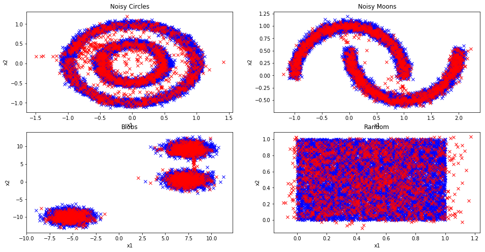
Figure 4: Sampling using Real NVP from toy 2D datasets (blue training data; red sample generated from Real NVP)
5.2 Image Datasets
I also implemented results on MNIST, CIFAR10, and CELEBA using similar preprocessing and setup to [1] (horizontal flips for all of them and cropping for CELEBA). The bits / dim for the experiments are shown in Table 1 with the comparison to [1] (and another normalizing flow model GLOW in the case of MNIST).
Dataset |
RealNVP (mine) |
RealNVP (paper) [1] |
|---|---|---|
MNIST |
1.92 |
1.26 (GLOW) |
CIFAR10 |
3.79 |
3.49 |
CELEBA |
3.25 |
3.02 |
My results are obviously far from state of the art but not that far off. To be fair, I didn't really spend much time hyper parameter tuning or configuring the training (e.g. epochs, learning rate). I also had a tiny GPU (my good old GTX1070), so I couldn't use the same batch sizes that were stated in the paper (assuming that made a difference). I probably could have gotten much closer to the paper if I had a bigger GPU and did a sweep of hyperparameters with some random seeds (which I assume all of these types of papers do). I'm pretty happy with the results though since in the past I've been much further from the published results.
Figure 5-7 show some random (non-handpicked) examples for MNIST, CIFAR10, and CELEBA respectively. Starting with Figure 5, the hand written digits of MNIST seem a bit off. You can seem some clear digits, and then some that are incomprehensible. One interesting thing to note is that each of the digits is sharp. This is in contrast to VAEs which usually are more blurry. In the end, the results aren't great but perhaps Real NVP doesn't perform as well in these cases (or maybe I need to train more)?
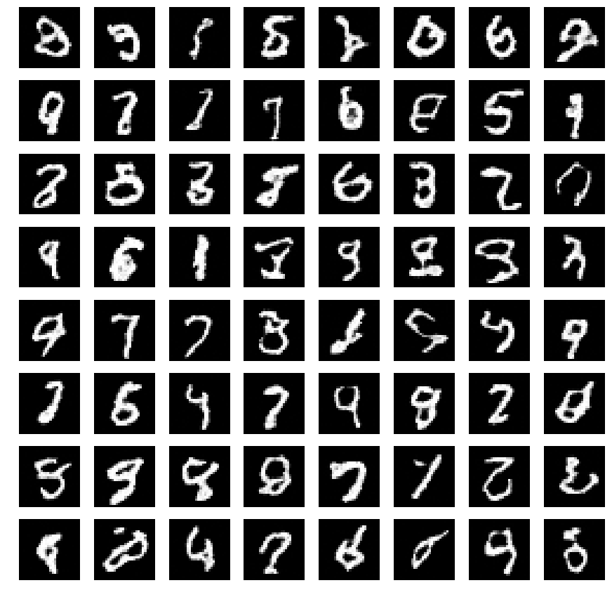
Figure 5: MNIST generated images
Next up are my CIFAR10 images in Figure 6. These ones look non-specific, which is typical for CIFAR10 (as far as I can tell by zooming in on pictures generated from papers). Qualitatively they don't look that far off from the samples published in [1]. The only comment I can really make is that the diversity of colours and shapes/objects isn't bad. This implies that the network is learning something.
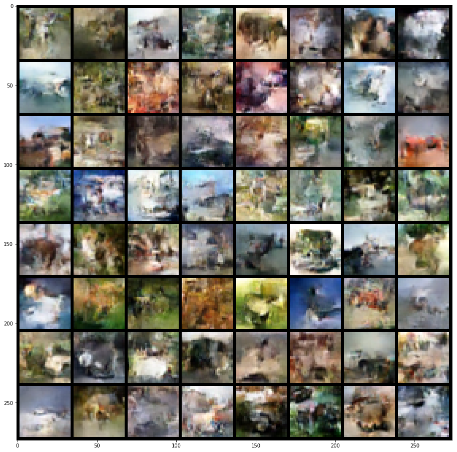
Figure 6: CIFAR10 generated images
Finally, I decided to use CELEBA (Figure 7), which is my first time training on this dataset. I've avoided it in the past because of my tiny 8GB GPU. Fortunately, I was able to barely fit it into memory (by using a smaller batch size). The samples are pretty bad. You can definitely make out faces but there are obvious places of corruption and the facial details are blurry. I suppose that more training might help improve things, but I also suspect that the faces in the paper are cherry picked. So it's probably a combination of both to get nicer images as shown in the paper.
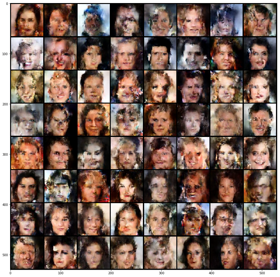
Figure 7: CELEBA generated images
6 Conclusion
I'm so happy that I was finally able to get this post out. I started playing around with Real NVP a while ago but I got frustrated trying to get it to work in Keras, so I got distracted with some other stuff (see my previous posts). Conceptually, I really enjoyed this topic because it was really surprising to me that such a simple transform works. Looking forward, I'm already pretty excited about a few papers that I've had my eye on and I can't wait to find some time to implement and write them up. Until next time!
7 Further Reading
Previous posts: A Note on Using Log-Likelihood for Generative Models
Wikipedia: Latent Variable Model, Probability Density Function, Inverse Transform Sampling, Probability Integral Transform, Change of Variables in the Probability Density Function
[1] Dinh, Sohl-Dickstein, Bengio, Density Estimation using Real NVP, arXiv:1605.08803, 2016
[2] Stanford CS236 Class Notes, https://deepgenerativemodels.github.io/notes/flow/
- 1
-
Apparently, autoregressive models can be interpreted as flow-based models (see [2]) but it's not very intuitive to me so I like to think of them as their own separate thing.
- 2
-
My schedule consisted of usually 30-60 minutes in the evening when I actually had some free time. I did have some other bits of free time as well when I had some extra help around the house from my extended family. Most of my other time is taken up by my main job and family time.