Maximum Entropy Distributions
This post will talk about a method to find the probability distribution that best fits your given state of knowledge. Using the principle of maximum entropy and some testable information (e.g. the mean), you can find the distribution that makes the fewest assumptions about your data (the one with maximal information entropy). As you may have guessed, this is used often in Bayesian inference to determine prior distributions and also (at least implicitly) in natural language processing applications with maximum entropy (MaxEnt) classifiers (i.e. a multinomial logistic regression). As usual, I'll go through some intuition, some math, and some examples. Hope you find this topic as interesting as I do!
Information Entropy and Differential Entropy
There are plenty of ways to intuitively understand information entropy, I'll try to describe one that makes sense to me. If it doesn't quite make sense to you, I encourage you to find a few different sources until you can piece together a picture that you can internalize.
Let's first clarify two important points about terminology. First, information entropy is a distinct idea from the physics concept of thermodynamic entropy. There are parallels, and connections have been made between the two ideas, but it's probably best to initially to treat them as separate things. Second, the "information" part refers to information theory, which deals with sending messages (or symbols) over a channel. One crucial point for our explanation is that the "information" (of a data source) is modelled as a probability distribution. So everything we talk about is with respect to a probabilistic model of the data.
Now let's start from the basic idea of information. Wikipedia has a good article on Shannon's rationale for information, check it out for more details. I'll simplify it a bit to pick out the main points.
First, information was originally defined in the context of sending a message between a transmitter and receiver over a (potentially noisy) channel. Think about a situation where you are shouting messages to your friend across a large field. You are the transmitter, your friend the receiver, and the channel is this large field. We can model what your friend is hearing using probability.
For simplicity, let's say you are only shouting (or transmitting) letters of the alphabet (A-Z). We'll also assume that the message always transmits clearly (if not this will affect your probability distribution by adding noise). Let's take a look at a couple examples to get a feel for how information works:
Suppose you and your friend agree that you will always shout "A" ahead of time (or a priori). So when you actually do start shouting, how much information is being transmitted? None, because your friend knows exactly what you are saying. This is akin to modelling the probability of receiving "A" as 1, and all other letters as 0.
Suppose you and your friend agree, a priori, that you will being shouting letters in order from some English text. Which letter do you think would have more information, "E" or "Z"? Since we know "E" is the most common letter in the English language, we can usually guess when the next character is an "E". So we'll be less surprised when it happens, thus it has a relatively low amount of information that is being transmitted. Conversely, "Z" is an uncommon letter. So we would probably not guess that it's coming next and be surprised when it does, thus "Z" conveys more information than "E" in this situation. This is akin to modelling a probability distribution over the alphabet with probabilities proportional to the relative frequencies of letters occurring in the English language.
Another way of describing information is a measure of "surprise". If you are more surprised by the result then it has more information. Based on some desired mathematical properties shown in the box below, we can generalize this idea to define information as:
The base of the logarithm isn't too important since it will just adjust the value by a constant. A usual choice is base 2 which we'll usually call a "bit", or base \(e\), which we'll call a "nat".
Properties of Information
The definition of information came about based on certain reasonable properties we ideally have:
\(I(p_i)\) is anti-monotonic - information increases when the probability of an event decreases, and vice versa. If something almost always happens (e.g. the sun will rise tomorrow), then there is no surprise and you really haven't gained much information; or if something very rarely happens (e.g. a gigantic earth quake), then you will be surprised and more information is gained.
\(I(p_i=0)\) is undefined - for infinitesimally small probability events, you have a infinitely large amount of information.
\(I(p_i)\geq 0\) - information is non-negative.
\(I(p_i=1)=0\) - sure things don't give you any information.
\(I(p_i, p_j)=I(p_i) + I(p_j)\) - for independent events \(i\) and \(j\), information should be additive. That is, getting the information (for independent events) together, or separately, should be the same.
Now that we have an idea about the information of a single event, we can define entropy in the context of a probability distribution (over a set of events). For a given discrete probability distribution for random variable \(X\), we define entropy of \(X\) (denoted by \(H(X)\)) as the expected value of the information of \(X\):
Et voila! The usual (non-intuitive) definition of entropy we all know and love. Note: When any of the probabilities are \(p_i=0\), you replace \(0\log(0)\) with \(0\), which is consistent with the limit as \(p\) approaches to 0 from the right.
Entropy, then, is the average amount of information or surprise for an event in a probability distribution. Going back to our example above, when transmitting only "A"s, the information transmitted is 0 (because \(P(\text{"A"})=1\) and \(0\) for other letters), so the entropy is naturally 0. When transmitting English text, the entropy will be the average entropy using letter frequencies 1.
Example 1: Entropy of a fair coin.
For a random variable X corresponding to the toss of a fair coin we have, \(P(X=H)=p\) and \(P(X=T)=1-p\) with \(p=0.5\). Using Equation 2 (using base 2):
So one bit of information is transmitted with every observation of a fair coin toss. If we vary the value of \(p\), we get a symmetric curve shown in Figure 1. The more biased towards H or T, the less entropy (information/surprise) we get (on average).
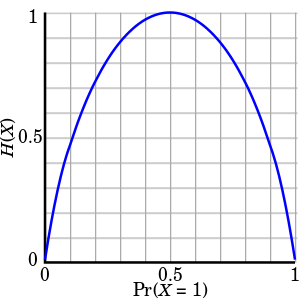
Figure 1: Entropy with varying \(p\) (source: Wikipedia)
A continuous analogue to (discrete) entropy is called differential entropy (or continuous entropy). It has a very similar equation using integrals instead of sums:
where it is understood that \(p(x)\log(p(x))=0\) when \(p(x)=0\). We have to be careful with differential entropy because some of the properties of (discrete) entropy do not apply to differential entropy, for example, differential entropy can be negative.
Principle of Maximum Entropy
The principle of maximum entropy states that given precisely stated prior data, the probability distribution that best represents the current state of knowledge is the one with the largest (information) entropy. In other words, if we only know certain statistics about the distribution, such as its mean, then this principle tells us that the best distribution to use is the one with the most surprise (more surprise, means fewer of your assumptions were satisfied). This rule can be thought of expressing epistemic modesty, or maximal ignorance, because it makes the least strong claim on a distribution beyond being informed by the prior data.
The precisely stated prior data should be in a testable form, which just means that given a probability distribution you say whether the statement is true or false. The most common examples are moments of a distribution such as the expected value or variance of a distribution, along with its support.
In terms of solving for these maximum entropy distributions, we can usually formulate it as maximizing a function (entropy) in the presence of multiple constraints. This is typically solved using Lagrange multipliers (see my previous post). Let's take a look at a bunch of examples to get a feel for how this works.
Example 2: Discrete Probability distribution with support \(\{a, a+1, \ldots, b-1, b\}\) with \(b > a\) and \(a,b \in \mathbb{Z}\).
First the function we're maximizing:
Next our constraints, which in this case is just our usual rule of probabilities summing to 1:
Using Lagrange multipliers, we can solve the Lagrangian by taking its partial derivatives and setting them to zero:
Solving for \(p_i\) and \(\lambda\):
So given no information about a discrete distribution, the maximal entropy distribution is just a uniform distribution. This matches with Laplace's principle of indifference which states that given mutually exclusive and exhaustive indistinguishable possibilities, each possibility should be assigned equal probability of \(\frac{1}{n}\).
Example 3: Jaynes' Dice
A die has been tossed a very large number N of times, and we are told that the average number of spots per toss was not 3.5, as we might expect from an honest die, but 4.5. Translate this information into a probability assignment \(p_n, n = 1, 2, \ldots, 6\), for the \(n\)-th face to come up on the next toss.
This problem is similar to the above except for two changes: our support is \(\{1,\ldots,6\}\) and the expectation of the die roll is \(4.5\). We can formulate the problem in a similar way with the following Lagrangian with an added term for the expected value (\(B\)):
Taking the partial derivatives and setting them to zero, we get:
Define a new quantity \(Z(\lambda_1)\) by substituting Equation 12 into 13:
Substituting Equation 12, and dividing Equation 14 by 13
Going back to Equation 12 and defining it in terms of \(Z\):
Unfortunately, now we're at an impasse because there is no closed form solution. Interesting to note that the solution is just an exponential-like distribution with parameter \(\lambda_1\) and \(Z(\lambda_1)\) as a normalization constant to make sure the probabilities sum to 1. Equation 16 gives us the desired value of \(\lambda_1\). We can easily find a solution using any root solver, such as the code below:
from numpy import exp
from scipy.optimize import newton

a, b, B = 1, 6, 4.5

# Equation 15
def z(lamb):
    return 1. / sum(exp(-k*lamb) for k in range(a, b + 1))

# Equation 16
def f(lamb, B=B):
    y = sum(k * exp(-k*lamb) for k in range(a, b + 1))
    return y * z(lamb) - B

# Equation 17
def p(k, lamb):
    return z(lamb) * exp(-k * lamb)

lamb = newton(f, x0=0.5)
print("Lambda = %.4f" % lamb)
for k in range(a, b + 1):
    print("p_%d = %.4f" % (k, p(k, lamb)))

# Output:
#   Lambda = -0.3710
#   p_1 = 0.0544
#   p_2 = 0.0788
#   p_3 = 0.1142
#   p_4 = 0.1654
#   p_5 = 0.2398
#   p_6 = 0.3475
The distribution is skewed much more towards \(6\). If you re-run the program with \(B=3.5\), you'll get a uniform distribution, which is what we would expect from a fair die.
Example 4: Continuous probability distribution with support \([a, b]\) with \(b > a\).
This is the continuous analogue to Example 2, so we'll use differential entropy instead of the discrete version along with the corresponding probability constraint of summing to \(1\) (\(p(x)\) is our density function):
Gives us the continuous analogue to the Lagrangian:
Notice that the problem is different from Example 1: we're trying to find a function that maximizes Equation 20, not just a discrete set of values. To solve this, we have to use the calculus of variations, which basically is the analogue to the value-maximization mathematics of regular calculus.
Describing variational calculus is a bit beyond the scope of this post (that's for next time!) but in this specific case, it turns out the equations look almost identical to Example 2. Taking the partial functional derivatives of Equation 20 and solving for the function:
So no surprises here, we get a uniform distribution on the interval \([a,b]\), analogous to the discrete version.
Wikipedia has a table of some common maximum entropy distributions, here are few you might encounter:
Support \(\{0, 1\}\) with \(E(x)=p\): Bernoulli distribution
Support \(\{1, 2, 3, \ldots\}\) with \(E(x)=\frac{1}{p}\): geometric distribution
Support \((0, \infty)\) with \(E(x)=b\): exponential distribution.
Support \((-\infty, \infty)\) with \(E(|x-\mu|)=b\): Laplacian distribution
Support \((-\infty, \infty)\) with \(E(x)=\mu, Var(x)=\sigma^2\): normal distribution
Support \((0, \infty)\) with \(E(\log(x))=\mu, E((\log(x) - \mu)^2)=\sigma^2\): lognormal distribution
Conclusion
The maximum entropy distribution is a very nice concept: if you don't know anything except for the stated data, assume the least informative distribution. Practically, it can be used for Bayesian priors but on a more philosophical note the idea has been used by Jaynes to show that thermodynamic entropy (in statistical mechanics) is the same concept as information entropy. Even though it's controversial, it's kind of reassuring to note that nature may be Bayesian. I don't know about you but this somehow makes me sleep more soundly at night :)
Further Reading
Wikipedia: Maximum Entropy Probability Distribution, Principle of Maximum Entropy, Entropy, Self-Information <https://en.wikipedia.org/wiki/Self-information#Definition>
"The Brandeis Dice Problem & Statistical Mechanics", Steven J. van Enk., arxiv 1408.6803.
- 1
-
This isn't exactly right because beyond the letter frequencies, we also can predict what the word is, which will change the information and entropy. Natural language also has redundancies such as "q must always be followed by u", so this will change our probability distribution. See Entropy and Redundancy in English for more details.