Bayesian Learning via Stochastic Gradient Langevin Dynamics and Bayes by Backprop
After a long digression, I'm finally back to one of the main lines of research that I wanted to write about. The two main ideas in this post are not that recent but have been quite impactful (one of the papers won a recent ICML test of time award). They address two of the topics that are near and dear to my heart: Bayesian learning and scalability. Dare I even ask who wouldn't be interested in the intersection of these topics?
This post is about two techniques to perform scalable Bayesian inference. They both address the problem using stochastic gradient descent (SGD) but in very different ways. One leverages the observation that SGD plus some noise will converge to Bayesian posterior sampling [Welling2011], while the other generalizes the "reparameterization trick" from variational autoencoders to enable non-Gaussian posterior approximations [Blundell2015]. Both are easily implemented in the modern deep learning toolkit thus benefit from the massive scalability of that toolchain. As usual, I will go over the necessary background (or refer you to my previous posts), intuition, some math, and a couple of toy examples that I implemented.
Table of Contents
1 Motivation
Bayesian learning is all about learning the posterior distribution for the parameters of your statistical model, which in turns allows you to quantify the uncertainty about them. The classic place to start is with Bayes' theorem:
where \({\bf x}\) is a vector of data points (often IID) and \({\bf \theta}\) is the vector of statistical parameters of your model.
In the general case, there is no closed form solution and you have to resort to heavy methods such as Markov Chain Monte Carlo (MCMC) or some form of approximation (which we'll get to later). MCMC methods never give you a closed form but instead give you samples from the posterior distribution, which you can use then use to compute any statistic you like. These methods are quite slow because they rely on Monte Carlo methods.
This brings us to our first scalability problem Bayesian learning: it does not scale well with the number of parameters. Randomly sampling with MCMC implies that you have to "explore" the parameter space, which potentially grows exponentially with the number of parameters. There are many techniques to make this more efficient but ultimately it's hard to overcome an exponential. The natural example for this situation is neural networks which can have orders of magnitude more parameters compared to classic Bayesian learning problems (I'll also add that the use-case of the posterior is usually different too).
The other non-obvious scalability issue with MCMC in Equation 1 is the data. Each evaluation of MCMC requires an evaluation of the likelihood and prior from Equation 1. For large data (e.g. modern deep learning datasets), you quickly hit issues with either memory and/or computation speed.
For non-Bayesian learning, modern deep learning has solved both of these problems by leveraging one of the simplest optimization methods out there (stochastic gradient descent) along with the massive compute power of modern hardware (and its associated toolchain). How can we leverage these developments to scale Bayesian learning? Keep reading to find out!
2 Background
2.1 Bayesian Networks and Bayesian Hierarchical Models
We can take the idea of parameters and priors from Equation 1 to multiple levels. Equation 1 implicitly assumes that there is one "level" of parameters (\(\theta\)) that we're trying to estimate with prior distributions (\(p({\bf \theta})\)) attached to them but there's no reason why you only need a single level. In fact, our parameters can be conditioned on parameters, which can be conditioned on parameters, and so on. This is called Bayesian hierarchical modelling. If this sounds oddly familiar, it's the same thing as Bayesian networks in a different context (if you're familiar with that). My previous post gives a high level summary on the intuition with latent variables.
To quickly summarize, in a parameterized statistical model there are broadly two types of variables: observed and unobserved. Observed variables are ones that we have values for and form our dataset; unobserved variables are ones we don't have values for, and can go by several names. In Bayesian networks they are usually called latent or hidden (random) variables, which can have complex conditional dependencies specified as a DAG. In hierarchical models they are called hyperparameters, which are the parameters of the observed models, the parameters of parameters, parameters of parameters of parameters and so on. Similarly, each of these hyperparameters has a distribution which we call a hyperprior. (Note: this is not the same concept as hyperparameters as it is usually used in the ML settings, which is very confusing.)
Latent variables and hyperparameters are mathematically the same and (from what I gather) the difference is really just in their interpretation. In the context of hierarchical models, the hyperparameters and hyperpriors represent some structural knowledge about the problem, hence of the use of term "priors". The data is typically believed to appear in hierarchical "clusters" that share similar attributes (i.e., drawn from the same distribution). This view is more typical in Bayesian statistics applications where the number of stages (and thus variables) is usually small (two or three). If terms such as fixed or random effects models ring a bell then this framing will make much more sense.
In Bayesian networks, the latent variables can represent the underlying phenomenon but also can be artificially introduced to make the problem more tractable. This happens more often in machine learning such as in variational autoencoders. In these contexts, they are often modelling a much bigger network and can have an arbitrarily number of stages and nodes. By varying assumptions on the latent variables and their connectivity, there are many efficient algorithms that can perform either approximate or exact inference on them. Most applications in ML seem to follow the Bayesian networks nomenclature since its context is more general. We'll stick with this framing since most of the ML sources will explain it this way.
2.2 Markov Chain Monte Carlo and Hamiltonian Monte Carlo
This subsection gives a brief introduction Monte Carlo Markov Chains (MCMC) and Hamiltonian Monte Carlo. I've written about both here and here if you want the nitty gritty details (and better intuition).
MCMC methods are a class of algorithm for sampling from a target probability distribution (e.g., posterior distribution). The most basic algorithm is relatively simple, starting from a given point:
Initial the current point to some random starting point (i.e., state)
Propose a new point (i.e., state)
With some probability calculated using the target distribution (or some function proportional to it), either (a) transition and accept this new point (i.e., state), or (b) stay at the current point (i.e., state).
Repeat steps 1 and 2, and periodically output the current point (i.e., state).
Many MCMC algorithms follow this general framework. The key is ensuring that the proposal and the acceptance probability define a Markov chain such that its stationary distribution (i.e., steady state) is the same as your target distribution. See my previous post on MCMC for more details.
There are two complications with this approach. The first complication is that your initial state may be in some weird region that causes the algorithm to explore parts of the state space that are low probability. To solve this, you can perform "burn-in" by starting the algorithm and throwing away a bunch of states to have a higher change to be in a more "normal" region of the state space. The other complication is that sequential samples will often be correlated, but you almost always want independent samples. Thus (as specified in the steps above), we only periodically output the current state as a sample to ensure that the we have minimal correlation. This is generally called "thinning". A well tuned MCMC algorithm will have both a high acceptance rate and little correlation between samples.
Hamiltonian Monte Carlo (HMC) is a popular MCMC algorithm that has a high acceptance rate with low correlation between samples. At a high level, it transforms the sampling of a target probability distribution into a physics problem with Hamiltonian dynamics. Intuitively, the problem is similar to a frictionless puck moving along a surface representing our target distribution. The position variables \(q\) represent the state from our probability distribution, and the momentum \(p\) (equivalently velocity) are a set of instrument variables to make the problem work. For each proposal point, we randomly pick a new momentum (and thus energy level of the system) and simulate from our current point. The end point is our new proposal point.
This is effectively simulating the associated differential equations of this physical system. It works well because the produced proposal point has both a high acceptance rate and can easily be "far away" with more simulation steps (thus low correlation). In fact, the acceptance rate would be 100% if it not for the fact that we have some discretization error from simulating the differential equations. See my previous post on HMC for more details.
A common method for simulation of this physics problem uses the "leap frog" method where we discretize time and simulate time step-by-step:
Where \(i\) is the dimension index, \(q(t)\) represent the position variables at time \(t\), \(p(t)\) similarly represent the momentum variables, \(\epsilon\) is the step size of the discretized simulation, and \(H := U(q) + K(p)\) is the Hamiltonian, which (in this case) equals the sum of potential energy \(U(q)\) and the kinetic energy \(K(p)\). The potential energy is typically the negative logarithm of the target density up to a constant \(f({\bf q})\), and the kinetic energy is usually defined as independent zero-mean Gaussians with variances \(m_i\):
Once we have a new proposal state \((q^*, p^*)\), we accept the new state according to this probability using a Metropolis-Hasting update:
2.3 Langevin Monte Carlo
Langevin Monte Carlo (LMC) [Radford2012] is a special case of HMC where we only take a single step in the simulation to propose a new state (versus multiple steps in a typical HMC algorithm). It is sometimes referred to as the Metropolis-Adjusted-Langevin algorithm (MALA) (see [Teh2015] for more details). With some simplification, we will see that a new familiar behaviour emerges from this special case.
Suppose we define kinetic energy as \(K(p) = \frac{1}{2}\sum p_i^2\), which is typical for a HMC formulation. Next, we set our momentum \(p\) as a sample from a zero mean, unit variance Gaussian (still same as HMC). Finally, we run a single step of the leap frog to get new a new proposal state \(q^*\) and \(p^*\).
We only need to focus on the position \(q\) because we resample the momentum \(p\) on each new proposal state so the simulated momentum \(p^*\) gets thrown away anyways. Starting from Equation 3:
Equation 7 is known in physics as (one type of) Langevin Equation (see box below for explanation), thus the name Langevin Monte Carlo.
Now that we have a proposal state (\(q^*\)), we can view the algorithm as running a vanilla Metropolis-Hastings update where the proposal is coming from a Gaussian with mean \(q_i(t) - \frac{\epsilon^2}{2} \frac{\partial U}{\partial q_i}(q(t))\) and variance \(\epsilon^2\) corresponding to Equation 7. By eliminating \(p\) (and the associated \(p^*\), not shown here) from the original HMC acceptance probability in Equation 6, we can derive the following expression:
Even though LMC is derived from HMC, its properties are quite different. The movement between states will be a combination of the \(\frac{\epsilon^2}{2} \frac{\partial U}{\partial q_i}(q(t))\) term and the \(\epsilon p(t)\) term. Since \(\epsilon\) is necessarily small (otherwise your simulation will not be accurate), the former term will be very small and the latter term will resemble a simple Metropolis-Hastings random walk. A big difference though is that LMC has better scaling properties when increasing dimensions compared to a pure random walk. See [Radford2012] for more details.
Finally, we'll want to re-write Equation 7 using different notation to line up with our usual notation for stochastic gradient descent. First, we'll use \(\theta\) instead of \(q\) to imply that we're sampling from parameters of our model. Next, we'll rewrite the potential energy \(U(\theta)\) as the likelihood times prior (where \(x_i\) are our observed data points):
Simplifying our Equation 7, we get:
Which looks eerily like gradient descent except that we're adding Gaussian noise at the end, stay tuned!
Langevin's Diffusion
In the field of stochastic differential equations, a general Itô diffusion process is of the form:
where \(X_t\) is a stochastic process, \(W_t\) is a Weiner process and \(a(\cdot), b(\cdot)\) are functions of \(X_t, t\). The form of Equation A.1 is the differential form. See my post on Stochastic Calculus for more details.
One of the forms of Langevin diffusion is a special case of Equation A.1:
Where \(q_t\) is the position, \(U\) is the potential energy, \(\frac{dU}{dq}\) is the force (position derivative of potential energy), and \(W_t\) is the Wiener process.
In the context of MCMC, we model the potential energy of this system as \(U(q) = \log f(q)\) where \(f\) is proportional to the likelihood times prior as is usually required in MCMC methods. With this substitution, Equation A.2 is the same as Equation 11 except a continuous time version of it. To see this more clearly, it is important to note that the increments of the standard Weiner process \(W_t\) are zero-mean Gaussians with variance equal to the time difference. Once discretized with step size \(\epsilon\), this precisely equals our \(\varepsilon\) sample from Equation 10.
2.4 Stochastic Gradient Descent and RMSprop
I'll only briefly cover stochastic gradient descent because I'm assuming most readers will be very familiar with this algorithm. Stochastic gradient descent (SGD) is an iterative stochastic optimization of gradient descent. The main difference is that it uses a randomly selected subset of the data to estimate the gradient at each step. For a given statistical model with parameters \(\theta\), log prior \(\log p(\theta)\), and log likelihood \(\sum_{i=1}^N \log[p(x_i | \theta_t)]]\) with observed data points \(x_i\), we have:
where \(\epsilon_t\) is a sequence of step sizes, and each iteration \(t\) we have a subset of \(n\) data points called a mini-batch \(X_t = \{x_{t_1}, \ldots, x_{t_n}\}\). By using an approximate gradient over many iterations the entire dataset is eventually used, and the noise in the estimated gradient averages out. Additionally for large datasets where the estimated gradient is accurate enough, this gives significant computational savings versus using the whole dataset at each iteration.
Convergence to a local optimum is guaranteed with some mild assumptions combined with a major requirement that the step size schedule \(\epsilon_t\) satisfies:
Intuitively, the first constraint ensures that we make progress to reaching the local optimum, while the second constraint ensures we don't just bounce around that optimum. A typical schedule to ensure that this is the case is using a decayed polynomial:
with \(\gamma \in (0.5, 1]\).
One of the issues with using vanilla SGD is that the gradients of the model parameters (i.e. dimensions) may have wildly different variances. For example, one parameter may be smoothly descending at a constant rate while another may be bouncing around quite a bit (especially with mini-batches). To solve this, many variations on SGD have been proposed that adjust the algorithm to account for the variation in parameter gradients.
RMSprop is a popular variant that is conceptually quite simple. It adjusts the learning rate per parameter to ensure that all of the learning rates are roughly the same magnitude. It does this by keeping a moving average (\(v(\theta, t)\)) of the squares of the magnitudes of recent gradients for parameter \(\theta\). For \(j^{th}\) parameter \(\theta^j\) in iteration \(t\), we have:
where \(Q_i\) is the loss function, and \(\gamma\) is the smoothing constant of the moving average with a typical value set at 0.99. With \(v(\theta^j, t)\), the update becomes:
From Equation 15, when you have large recent gradients (\(v(\theta^j, t) > 1\)), it scales the learning rate down; while if you have small recent gradients (\(v(\theta^j, t) < 1\)), it scales the learning rate up. If recently \(\nabla Q\) is constant in each parameter but with different magnitudes, it will update each parameter by the learning rate \(\epsilon_t\), attempting to descend each dimension at the same rate. Empirically, these variations of SGD are necessary to make SGD practical for a wide range of models.
2.5 Variational Inference and the Reparameterization Trick
I've written a lot about variational inference in past posts so I'll keep this section brief and only touch upon the relevant parts. If you want more detail and intuition, check out my posts on Semi-supervised learning with Variational Autoencoders, and Variational Bayes and The Mean-Field Approximation.
As we discussed above, our goal is to find the posterior, \(p(\theta|X)\), that tells us the distribution of the \(\theta\) parameters. Unfortunately, this problem is intractable for all but the simplest problems. How can we overcome this problem? Approximation!
We'll approximate \(p(\theta|X)\) by another known distribution \(q(\theta|\phi)\) parameterized by \(\phi\). Importantly, \(q(\theta|\phi)\) often has simplifying assumptions about its relationships with other variables. For example, you might assume that they are all independent of each other e.g., \(q(\theta|\phi) = \prod_{i=1}^n q_i(\theta_i|\phi_i)\) (a example of mean-field approximation).
The nice thing about this approximation is that we turned our intractable Bayesian learning problem into an optimization one where we just want to find the parameters \(\phi\) of \(q(\theta|\phi)\) that best match our posterior \(p(\theta|X)\). How well our approximation matches our posterior is both dependent on the functional form of \(q\) as well as our optimization procedure.
In terms of "best match", the standard way of measuring it is to use KL divergence. Without going into the derivation (see my previous post), if we start from the KL divergence between our approximate posterior and exact posterior, we'll arrive at the evidence lower bound (ELBO) for a single data point \(X\):
The left hand side of Equation 16 is constant (with respect to the observed data), so maximizing the right hand side achieves our desired goal. It just so happens this looks a lot like finding a MAP with a likelihood and prior term except for two differences: (a) we have an additional term for our approximate posterior, and (b) we have to take the expectation with respect to samples from that approximate posterior. When using a SGD approach, we can sample points from the \(q\) distribution and use it to approximate the expectation in Equation 16. In many cases though, it's not obvious how to sample from \(q\) because you also need to backprop through it.
In the case of variational autoencoders, we define an approximate Gaussian posterior \(q(z|\phi)\) on the latent variables \(z\). This approximate posterior is defined by a neural network with weights \(\phi\) that output a mean and variance representing the parameters of the Gaussian. We will want to sample from \(q\) to approximate the expectation in Equation 16, but also backprop through \(q\) to update the weights \(\phi\) of the approximate posterior. You can't directly backprop through it but you can reparameterize it by using a standard normal distribution, starting from Equation 16 (using \(z\) instead of \(\theta\)):
where \(\mu_z\) and \(\Sigma_z\) are the mean and covariance matrix of the approximate posterior, and \(\epsilon\) is a sample from a standard Gaussian. This is commonly referred to as the "reparameterization trick" where instead of directly computing \(z\) you just scale and shift a standard normal distribution using the mean and covariances. Thus, you can still backprop through \(z\) to optimize the mean/covariance networks. The last line approximates the expectation by taking a single sample, which often works fine when using SGD.
3 Stochastic Gradient Langevin Dynamics
Stochastic Gradient Langevin Dynamics (SGLD) combines the ideas of Langevin Monte Carlo (Equation 10) with Stochastic Gradient Descent (Equation 11) given by:
This results in an algorithm that is mechanically equivalent to SGD except with some Gaussian noise added to each parameter update. Importantly though, there are several key choices that SGLD makes:
\(\epsilon_t\) decreases towards zero just as in SGD.
Balance the Gaussian noise \(\varepsilon\) variance with the step size \(\epsilon_t\) as in LMC.
Ignore the Metropolis-Hastings updates (Equation 8) using the fact that rejection rates asymptotically go to zero as \(\epsilon_t \to 0\).
This algorithm has the advantage of SGD of being able to work on large data sets (because of the mini-batches) while still computing uncertainty (using LMC-like estimates). The avoidance of the Metropolis-Hastings update is key so that an expensive evaluation of the whole dataset is not needed at each iteration.
The intuition here is that in earlier iterations this will behave much like SGD stepping towards a local minimum because the large gradient overcomes the noise. In later iterations with a small \(\epsilon_t\), the noise dominates and the gradient plays a much smaller role, resulting in each iteration bouncing around the local minimum via a random walk (with a bias towards the local minimum from the gradient). Additionally, in between these two extremes the algorithm should vary smoothly. Thus with carefully selected hyperparameters, you can effectively sample from the posterior distribution (more on this later).
What is not obvious though is that why this should give correct the correct result. It surely will be able to get close to a local minimum (similar to SGD) but why would it give the correct uncertainty estimates without the Metropolis-Hastings update step? This is the topic of the next subsection.
3.1 Correctness of SGLD
Note: [Teh2015] has the hardcore proof of SGLD correctness versus a very informal sketch presented in the original paper ([Welling2011]) . I'll mainly stick to the original paper's presentation (mostly because the hardcore proof is way beyond my comprehension), but will call out a couple of notable things from the formal proof.
To set up this problem, let us first define several quantities. First define the true gradient of the log probability, which is just the negative gradient our usual MAP loss function (with no mini-batches):
Next, let's define another related quantity:
Equation 20 is essentially the difference between our SGD update (with mini-batch \(t\)) and the true gradient update (with all the data). Notice that \(h_t(\theta) + g(\theta)\) is just an SGD update which can be obtained by cancelling out the last term in \(h_t(\theta)\).
Importantly, \(h_t(\theta)\) is a zero-mean random variable with finite variance \(V(\theta)\). Zero-mean because we're subtracting out the true gradient so our random mini-batches should not have any bias. Similarly, the randomness comes from the fact that we're randomly selecting finite mini-batches, which should yield only a finite variance.
With these quantities, we can rewrite Equation 18 using the fact that \(h_t(\theta) + g(\theta)\) is an SGD update:
With the above setup, we'll show two statements:
Transition: When we have large \(t\), the SGLD state transition of Equation 18/21 will approach LMC, that is, have its equilibrium distribution be the posterior distribution.
Convergence: There exists a subsequence of \(\theta_1, \theta_2, \ldots\) of SGLD that converges to the posterior distribution.
With these two shown, we can see that SGLD (for large \(t\)) will eventually get into a state where we can theoretically sample the posterior distribution by taking the appropriate subsequence. The paper makes a stronger argument that the subsequence convergence implies convergence of the entire sequence but it's not clear to me that it is the case. At the end of this subsection, I'll also mention a theorem from the rigorous proof ([Teh2015]) that gives a practical result where this may not matter.
Transition
We'll argue that Equation 18/21 converges to the same transition probability as LMC and thus its equilibrium distribution will be the posterior.
First notice that Equation 18/21 is the same equation as LMC (Equation 10) except for the additional randomness due to the mini-batches: \(\frac{N}{n} \sum_{i=1}^n \nabla \log[p(x_{ti} | \theta_t)]\). This term is multiplied by a \(\frac{\epsilon_t}{2}\) factor whereas the standard deviation from the \(\varepsilon\) term is \(\sqrt{\epsilon_t}\). Thus as \(\epsilon_t \to 0\), the error from the mini-batch term will vanish faster than the \(\varepsilon\) term, converging to the LMC proposal distribution (Equation 10). That is, at large \(t\) it approximates LMC and eventually converges to it in the limit since the gradient update (and the difference between the two) vanishes.
Next, we observe that LMC is a special case of HMC. HMC is actually a discretization of a continuous time differential equation. The discretization introduces error in the calculation, which is the only reason why we need a Metropolis-Hastings update (see previous post on HMC). However as \(\epsilon_t \to 0\), this error becomes negligible converging to the HMC continuous time dynamics, implying a 100% acceptance rate. Thus, there is no need for an MH update for very small \(\epsilon_t\).
In summary for large \(t\), the \(t^{th}\) iteration of Equation 18/21 closely approximates the LMC Markov chain transition with very small error so its equilibrium distribution closely approximates the desired posterior. This would be great if we had a fixed \(t\) but we are shrinking \(t\) towards 0 (as is needed by SGD), thus SGLD actually defines a non-stationary Markov Chain, and so we still need to show the actual sequence will converge to the posterior.
Convergence
We will show that there exists some sequence of samples \(\theta_{t=a_1}, \theta_{t=a_2}, \ldots\) that converge to the posterior for some strictly increasing sequence \(a_1, a_2, \ldots\) (note: the sequence is not sequential e.g., \(a_{n+1}\) is likely much bigger than \(a_{n}\)).
First we fix a small \(\epsilon_0\) such that \(0 < \epsilon_0 << 1\). Assuming \(\{\epsilon_t\}\) satisfy the decayed polynomial property from Equation 13, there exists an increasing subsequence \(\{a_n \}\) such that \(\sum_{t=a_n+1}^{a_{n+1}} \epsilon_t \to \epsilon_0\) as \(n \to \infty\) (note: the \(+1\) in the sum's upper limit is in the subscript, while the lower limit is not). That is, we can split the sequence \(\{\epsilon_t\}\) into non-overlapping segments such that successive segments approaches \(\epsilon_0\). This can be easily constructed by continually extending the current run until you go over \(\epsilon_0\). Since \(\epsilon_t\) is decreasing, and we are guaranteed that the sequence doesn't converge (Equation 12), we can always construct the next segment with a smaller error than the previous one.
For large \(n\), if we look at each segment \(\sum_{t=a_n+1}^{a_{n+1}} \epsilon_t\), the total Gaussian noise injected will be the sum of each of the Gaussian noise injections. The variance of sums of independent Gaussians is just the sum of the variances, so the total variance will be \(O(\epsilon_0)\). Thus, the injected noise (standard deviation) will be on the order of \(O(\sqrt{\epsilon_0})\). Given this, next we will want to show that the variance from the mini-batch error is dominated by this injected noise.
To start, since \(\epsilon_0 << 1\), we have \(||\theta_t-\theta_{t=a_n}|| << 1\) for \(t \in (a_n, a_{n+1}]\) since the updates from Equation 18/21 cannot stray too far from where it started. Assuming the gradients vary smoothly (a key assumption) then we can see the total update without the injected noise for a segment \(t \in (a_n, a_{n+1}]\) is (i.e., Equation 21 minus the noise \(\varepsilon\)):
We see that the \(g(\cdot)\) summation expands into the gradient at \(\theta_{t=a_n}\) plus an error term \(O(\epsilon_0)\). This is from our assumption of \(||\theta_t-\theta_{t=a_n}|| << 1\) plus the gradients varying smoothly (Lipschitz continuity), which imply that the difference between successive gradients will also be much smaller than 1 (for an appropriately small \(\epsilon_0\)). Thus, the error from this term on this segment will be \(\sum_{t=a_n+1}^{a_{n+1}} \frac{\epsilon_t}{2} O(1) = O(\epsilon_0)\) as shown in Equation 22.
Next, we deal with the \(h_t(\cdot)\) in Equation 22. Since we know that \(\theta_t\) did not vary much in our interval \(t \in (a_n, a_{n+1}]\) given our \(\epsilon_t << 1\) assumption, we have \(h_t(\theta_t) = O(1)\) in our interval since our gradients vary smoothly (again due to Lipschitz continuity). Additionally each \(h_t(\cdot)\) will be a random variable which we can assume to be independent, thus IID (doesn't change argument if they are randomly partitioned which will only make the error smaller). Plugging this into \(\sum_{t=a_n+1}^{a_{n+1}} \frac{\epsilon_t}{2} h_t(\theta_t)\), we see the variance is \(O(\sum_{t=a_n+1}^{a_{n+1}} (\frac{\epsilon_t}{2})^2)\). Putting this together in Equation 22, we get:
From Equation 22, we can see the total stochastic gradient over our segment is just the exact gradient starting from \(\theta_{t=a_n}\) with step size \(\epsilon_0\) plus a \(O(\epsilon_0)\) error term. But recall our injected noise was of order \(O(\sqrt{\epsilon_0})\), which in turn dominates \(O(\epsilon_0)\) (for \(\epsilon_0 < 1\)). Thus for small \(\epsilon_0\), our sequence \(\theta_{t=a_1}, \theta_{t=a_2}, \ldots\) will approximate LMC because each segment will essentially be an LMC update with very small, decreasing error. As a result, this subsequence will converge to the posterior as required.
Now the above argument showing that there exists a subsequence that samples from the posterior isn't that useful because we don't know what that subsequence is! But [Teh2015] provides a much more rigorous treatment of the subject showing a much more useful result in Theorem 7. Without going into all of the mathematical rigour, I'll present the basic idea (from what I can gather):
Theorem 1: (Summary of Theorem 7 from [Teh2015]) For a test function \(\varphi: \mathbb{R}^d \to \mathbb{R}\), the expectation of \(\varphi\) with respect to the exact posterior distribution \(\pi\) can be approximated by the weighted sum of \(m\) SGLD samples \(\theta_0 \ldots \theta_{m-1}\) that holds almost surely (given some assumptions):
\begin{equation*} \lim_{m\to\infty} \frac{\epsilon_1 \varphi(\theta_0) + \ldots + \epsilon_m \varphi(\theta_{m-1})}{\sum_{t=1}^m \epsilon_t} = \int_{\mathbb{R}^d} \varphi(\theta)\pi(d\theta) \tag{24} \end{equation*}
Theorem 1 gives us a more practical way to utilize the samples from SGLD. We don't need to generate the exact samples that we would get from LMC, instead we can just directly use the SGLD samples and their respective step sizes to compute a weighted average for any actual quantity we would want (e.g. expectation, variance, credible interval etc.). According to Theorem 1, this will converge to the exact quantity using the true posterior. See [Teh2015] for more details (if you dare!).
3.2 Preconditioning
One problem both with SGD and SGLD is that the gradients updates might be very slow due to the curvature of the loss surface. This is known to be a common phenomenon in large parameter models like neural networks where there are many saddle points. These parts of a surface have very small gradients (in at least one dimension), which will cause any SGD-based optimization procedure to be very slow. On the other end, if one of the dimensions in your loss has large curvature (and thus gradient), it could cause unnecessary oscillations in one dimension while the other one with low curvature crawls along. The solution to this problem is to use a preconditioner.
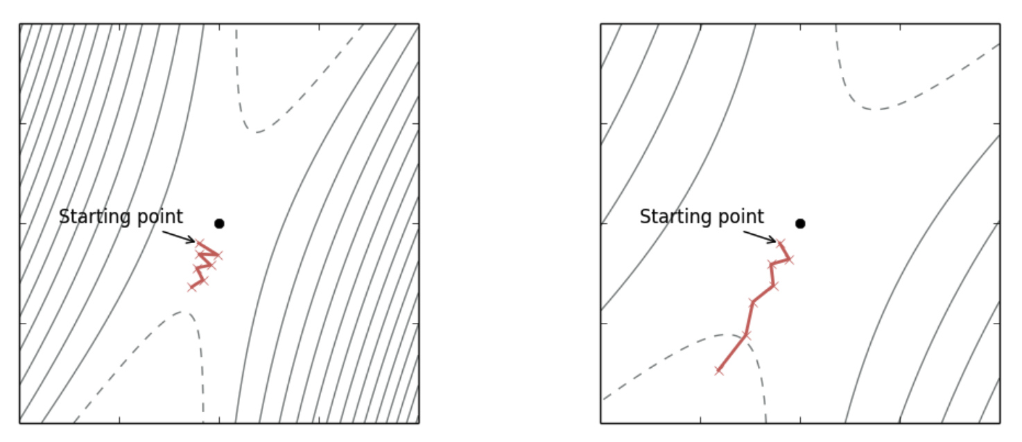
Figure 1: (Left) Original loss landscape, SGD converges slowly. (Right) Transformed loss landscape with a preconditioner with reduced oscillations and faster progress. Notice the contour lines are more evenly spaced out in each direction. (source: [Dauphin2015] )
Preconditioning is a type of local transform that changes the optimization landscape so the curvature is equal in all directions ([Dauphin2015]). As shown in Figure 1, preconditioning can transform the curvature (shown by the contour lines) and as a result make SGD converge more quickly. Formally, for a loss function \(f\) with parameters \(\theta \in \mathbb{R}^d\), we introduce a non-singular matrix \({\bf D}^{\frac{1}{2}}\) such that \(\hat{\theta}={\bf D}^{\frac{1}{2}}\theta\). Using the change of variables formula, we can define a new function \(\hat{f}(\hat{\theta})\) that is equivalent to our original function with its associated gradient (using the chain rule):
Thus, regular SGD can be performed on the original \(\theta\) (for convenience we'll define \({\bf G}={\bf D}^{-1}\)):
So the transformation turns out to be quite simple by multiplying our gradient with a user chosen preconditioning matrix \({\bf G}\) that is usually a function of the current parameters \(\theta_{t-1}\). In the context of SGLD, we have an equivalent result ([Li2016]) where \({\bf G}\) defines a Riemannian manifold:
where \(\Gamma(\theta_t) = \sum_j \frac{\partial G_{i,j}}{\partial \theta_j}\) describe how the preconditioner changes with respect to \(\theta_t\). Notice the preconditioner is applied to the noise as well.
Previous approaches to use a preconditioner relied on the expected Fisher information matrix, which is too costly for any modern deep learning model since it grows with the square of the number of parameters (similar to the Hessian). It turns out that we don't specifically need the Fisher information matrix, we just need something that defines the Riemannian manifold metric, which only requires a positive definite matrix.
The insight from [Li2016] was that we can use RMSprop as the preconditioning matrix since it satisfies the positive definite criteria, and has shown empirically to do well in SGD (being only a diagonal preconditioner matrix):
where \(v(\theta_{t+1})=v(\theta, t)\) from Equation 14 and \(\lambda\) is a small constant to prevent numerical instability.
Additionally, [Li2016] has shown that there is no need to include the \(\Gamma(\theta)\) term in Equation 27 (even though it's not too hard to compute for a diagonal matrix). This is because it introduces an additional bias term that scales with \(\frac{(1-\alpha)^2}{\alpha^3}\) (from Equation 27), which is practically always set close to 1 (e.g. PyTorch's default for RMSprop is \(\alpha = 0.99\)). As a result, we can simply use off-the-shelf RMSprop with only a slight adjustment to the SGLD noise and gain the benefits of preconditioning.
3.3 Practical Considerations
Besides preconditioning, SGLD has some other caveats inherited from MCMC. First your initial condition matters, so you likely want to run it for a while before you start sampling (i.e., "burn-in"). Similarly, adjacent samples (particularly with a random walk method such as LMC/SGLD) will be highly correlated so you will only want to take periodic samples to get (mostly) independent samples (although with Theorem 1 this may not be necessary) depending on your application. Finally, for both deep learning and MCMC, your hyperparameters matter a lot. For example, initial conditions, learning rate schedule, and priors all matter a lot. So while a lot of the above techniques help, there's no free lunch here.
4 Bayes by Backprop
Bayes by Backprop ([Blundell2015]) is a generalization of some previous work to allow an approximation of Bayesian uncertainty, particularly for weights in large scale neural network models where traditional MCMC methods do not scale. Approximation is the key word here as it utilizes variational inference (Equation 16). More precisely, instead of directly estimating the posterior, it preselects the functional form of a distribution (\(q(\theta|\phi)\)) parameterized by \(\phi\), and optimizes \(\phi\) using Equation 16. The right hand side of Equation 16 is often called the variational free energy (among other names), which we'll denote by \(\mathcal{F}(X, \phi)\):
Recall that instead of solving for point estimates of \(\theta\), we're trying to solve for \(\phi\), which implicitly gives us (approximate) distributions in the form of \(q(\theta|\phi)\). To make this concrete, for a neural network, \(\theta\) would be the weights and instead of a single number for each one, we would have a known distribution \(q(\theta|\phi)\) (that we select) parameterized by \(\phi\).
The main problem with Equation 29 is that we will need to sample from \(q(\theta|\phi)\) in order to approximate the expectation, but we will also need to backprop through the "sample" in order to optimize \(\phi\). If this sounds familiar, it is precisely the same issue we had with variation autoencoders. The solution there was to use the "reparameterization trick" to rewrite the expectation in terms of a standard Gaussian distribution (and some additional transformations) to yield an equivalent loss function that we can backprop through.
[Blundell2015] generalizes this concept beyond Gaussians to any distribution with the following proposition:
Proposition 1: (Proposition 1 from [Blundell2015]) Let \(\varepsilon\) be a random variable with probability density given by \(q(\varepsilon)\) and let \(\theta = t(\phi, \varepsilon)\) where \(t(\phi, \varepsilon)\) is a deterministic function. Suppose further that the marginal probability density of \(\theta\), \(q(\theta|\phi)\), is such that \(q(\varepsilon)d\varepsilon = q(\theta|\phi)d\theta\). Then for a function \(f(\cdot)\) with derivatives in \(\theta\):
\begin{equation*} \frac{\partial}{\partial\phi}E_{q(\theta|\phi)}[f(\theta,\phi)] = E_{q(\varepsilon)}\big[ \frac{\partial f(\theta,\phi)}{\partial\theta}\frac{\partial\theta}{\partial\phi} + \frac{\partial f(\theta, \phi)}{\partial \phi} \big] \tag{30} \end{equation*}Proof:
\begin{align*} \frac{\partial}{\partial\phi}E_{q(\theta|phi)}[f(\theta,\phi)] &= \frac{\partial}{\partial\phi}\int f(\theta,\phi)q(\theta|\phi)d\theta \\ &= \frac{\partial}{\partial\phi}\int f(\theta,\phi)q(\varepsilon)d\varepsilon && \text{Given in proposition}\\ &= \int \frac{\partial}{\partial\phi}[f(\theta,\phi)]q(\varepsilon)d\varepsilon \\ &= E_{q(\varepsilon)}\big[ \frac{\partial f(\theta,\phi)}{\partial\theta}\frac{\partial\theta}{\partial\phi} + \frac{\partial f(\theta, \phi)}{\partial \phi}\big] && \text{chain rule} \\ \tag{31} \end{align*}
So Proposition 1 tells us that the "reparameterization trick" is valid in the context of gradient based optimization (i.e., SGD) if we can show \(q(\varepsilon)d\varepsilon = q(\theta|\phi)d\theta\). Equation 30 may be a bit cryptic because of all the partial derivatives but notice two things. First, the expectation is now with respect to a standard distribution \(q(\varepsilon)\), and, second, the inner part of the expectation is done automatically through backprop when you implement \(t(\phi, \varepsilon)\) so you don't have to explicitly calculate it (it's just the chain rule). Let's take a look at a couple of examples.
First, let's take a look at the good old Gaussian distribution with parameters \(\phi = \{\mu, \sigma\}\) and \(\varepsilon\) being a standard Gaussian. We let \(t(\mu, \sigma, \varepsilon) = \sigma \cdot \varepsilon + \mu\). Thus, we have:
We can easily see that the two expressions are the same. To drive the point home, we can show the same relationship with the exponential distribution parameterized by \(\lambda\) using \(t(\lambda, \varepsilon) = \frac{\varepsilon}{\lambda}\) for standard exponential distribution \(\varepsilon\):
The nice thing about this trick is that it's widely implemented in modern tooling. For example, PyTorch has this implemented using the rsample() method (where applicable). You can look into each of the respective implementations to see how the \(t(\cdot)\) function is defined. See the Pathwise derivative section of the PyTorch docs for details.
With this reparameterization trick (and picking appropriate distributions), one can easily implement variational inference by substituting the exact posterior for a fixed parameterized distribution (e.g., Gaussian, exponential etc.). This allows you to easily train the network using standard SGD methods that sample from this approximate posterior distribution, but importantly can backprop through them to update the parameters of these approximate posteriors to hopefully achieve a good estimate of uncertainty. However this does have the same limitations as variational inference, which will often underestimate variance. So there's also no free lunch here either.
5 Experiments
5.1 Simple Gaussian Mixture Model
The first experiment I did was try to reproduce the simple mixture model with tied means from [Welling2011]. The model from the paper is specified as:
with \(p=0.5, \sigma_1^2=10, \sigma_2^2=1, \sigma_x^2=2\). They generate 100 \(x_i\) data points using a fixed \(\theta_1=0, \theta_2=1\). In the paper, they say that this generates a bimodal distribution but I wasn't able to reproduce it. I had to change \(\sigma_x^2=2.56\) to get a slightly wider bimodal distribution. I did this only for the data generation, all the training uses \(\sigma_x^2=2\). Theoretically, if they got a weird random seed they might be able to get something bimodal, but I wasn't able to. Figure 2 shows a histogram of the data I generated with the modified \(\sigma_x^2=2.56\).
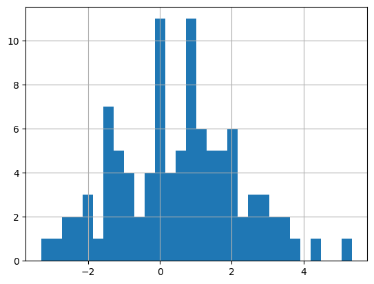
Figure 2: Histogram of \(x_i\) datapoints
From Equation 34, you can that the only parameters we need to estimate are \(\theta_1\) \(\theta_2\). If our procedure is correct, our posterior distribution should have a lot of density around \((\theta_1, \theta_2) = (0, 1)\).
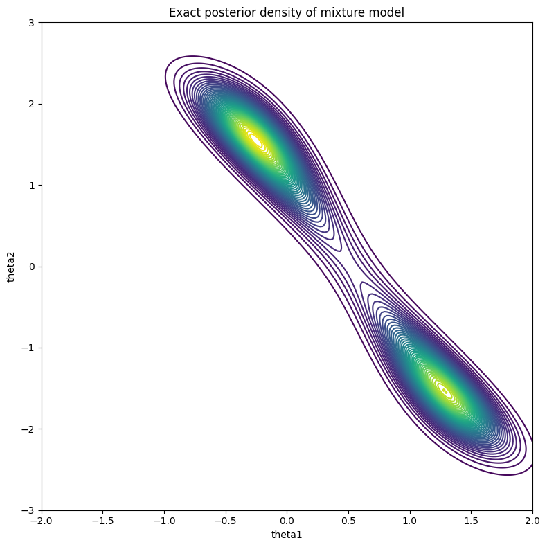
Figure 3: True posterior
Since this is just a relatively simple two dimensional problem, you can estimate the posterior by discretizing the space and calculating the unnormalized posterior (likelihood times prior) for each cell. As long as you don't overflow your floating point variables, you should be able to get a contour plot as shown in Figure 3. As you can see, the distribution is bimodal with a peak at \((-0.25, 1.5)\) and \((1.25, -1.5)\). It's not exactly the \((0, 1)\) peak we were expecting, but considering that we only sampled 100 points, this is the "best guess" based on the data we've seen (and the associated priors).
5.1.1 Results
Update 2023-08-17: Section updated with a bug fix, thanks @davetornado!
The first obvious thing to do is estimate the posterior using MCMC. I used PyMC for this because I think it has the most intuitive interface. The code is only a handful of lines and is made easy with the builtin NormalMixture distribution. I used the default NUTS sampler (extension of HMC) to generate 5000 samples with a 2000 sample burnin. Figure 4 shows the resulting contour plot, which line up very closely with the exact results in Figure 3.
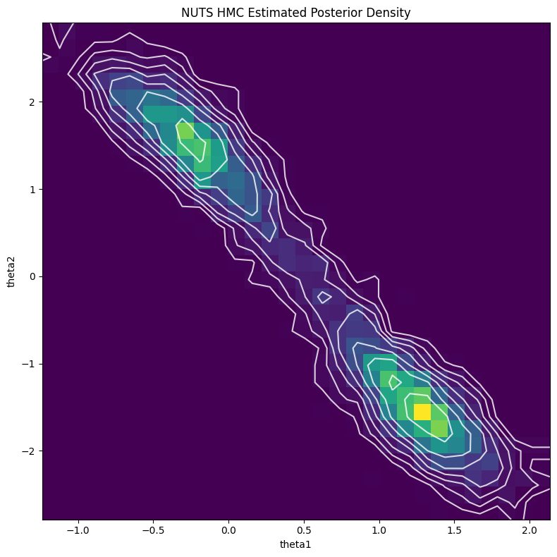
Figure 4: MCMC estimate of posterior
Next, I implemented both SGD and SGLD in PyTorch (using the same PyTorch Module). This was pretty simple by leveraging the builtin distributions package, particularly the MixtureSameFamily one.
For SGD with batch size of \(100\), learning rate (\(\epsilon\)) 0.01, 300 epochs, and initial values as \((\theta_1, \theta_2) = (1, 1)\), I was able to iterate towards a solution of \((-0.2327, 1.5129)\), which is pretty much our first mode from Figure 3. This gave me confidence that my model was correct.
Next, moving on to SGLD, I used the same effective decayed polynomial learning rate schedule as the paper with \(a=0.01, b=0.0001, \gamma=0.55\) that results in 10000 sweeps through the entire dataset with batch size of 1. I also did different experiments with batch size of 10 and 100, adjusting the same decaying polynomial schedule so that the total number of gradient updates are the same (see the notebook). I didn't do any burnin or thinning (although I probably should have?). The results are shown in Figure 5.
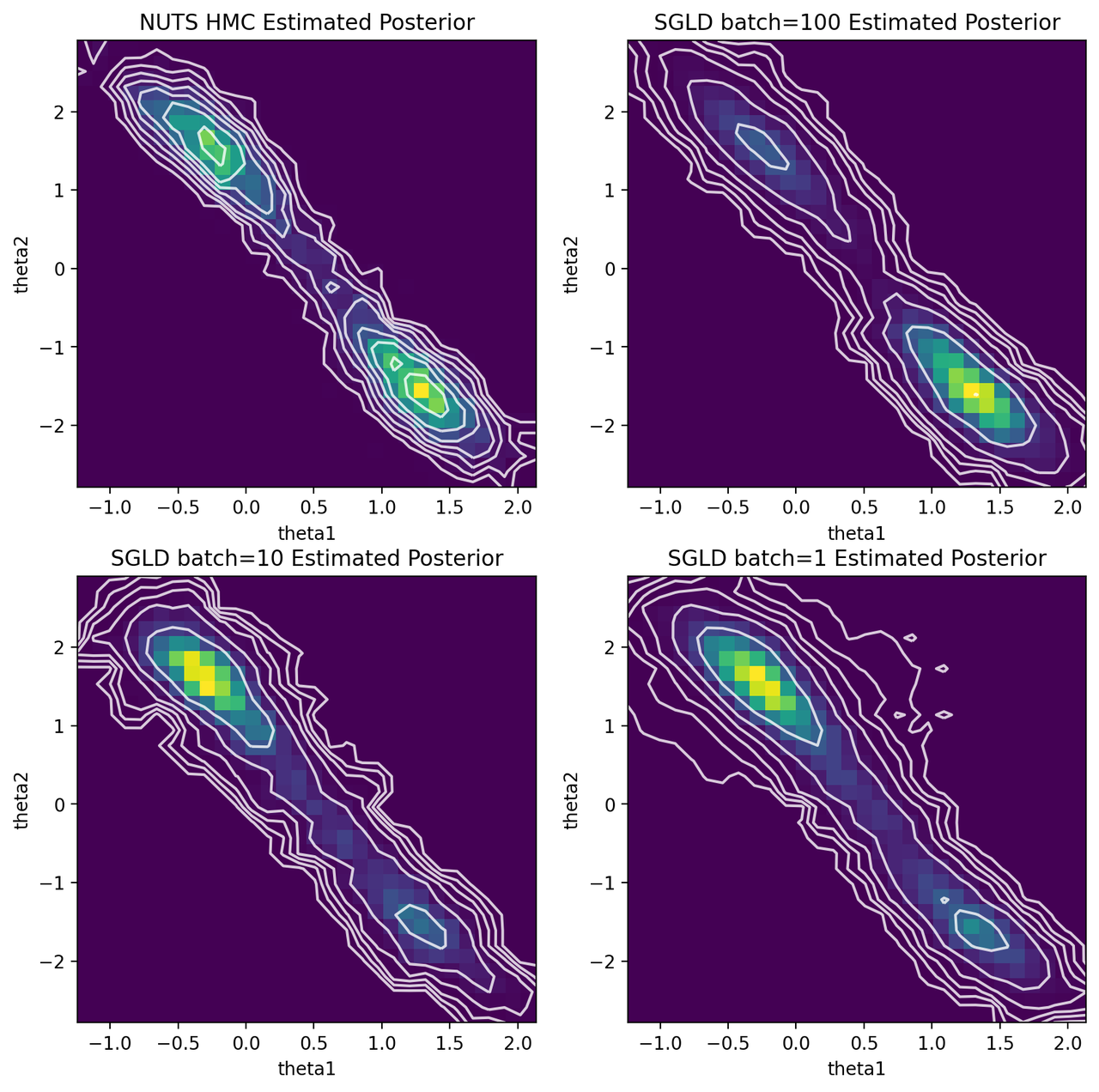
Figure 5: HMC and SGLD estimates of posterior for various batch sizes
We can see that SGLD is no panacea for posterior estimation. With batch size of 100, it spends most of its time in the bottom right mode, while mostly missing the top left one. It makes sense the SGLD using the polynomial learning rate schedule would have a tendency to sit in one mode because we're rapidly decaying \(\epsilon\) (and thus ability to "jump" around and find the other mode). The upside is that it seemed to the right shape and location of the distribution overall distribution for both modes.
Both batch size of 1 and 10 shows a similar story to that of 100 but this time they spend most of its time in the top left mode. Where SGLD gets "stuck" seems to depend on the initial conditions and the randomness injected. However, it does appear to have the right shape as with batch size 100.
My conclusion from this experiment is that vanilla SGLD is not as robust as MCMC. It's so sensitive to the learning rate schedule, which can cause it to have issues finding modes as seen above. There are numerous extensions to SGLD that I haven't really looked at (including ones that are inspired by HMC) so those may provide more robust algorithms to do at-scale posterior sampling. Having said that, perhaps you aren't too interested in trying to generate the exact posterior. In those cases, SGLD seems to do a good enough job at estimating the uncertainty around one of the modes (at least in this simple case).
5.2 Stochastic Volatility Model
The next experiment I did was with a stochastic volatility model from this example in the PyMC docs. This is actually kind of the opposite of what you would want to use SGLD and Bayes by Backprop for because it is a hierarchical model for stock prices with only a single time series, which is the observed price of the S&P 500. I mostly picked this model because I was curious how we could apply these methods to more complex hierarchical Bayesian models. Being one of the prime examples of where Bayesian methods can be used to analyze a problem, I naively thought that this would be an easy thing to model. It turned out to be much more complex than I expected as we shall see.
First, let's take a look at the definition of the model:
Equation 35 models the logarithm of the daily returns \(r_i\) with a student-t distribution, parameterized by the degrees of freedom \(\nu\) following an exponential distribution, and volatility \(s_i\) where \(i\) is the time index. The volatility follows a Gaussian random walk across all 2905 time steps, which is parameterized by a common variance given by an exponential distribution. To be clear, we are modelling the entire time series at once with a different log-return and volatility random variable for each time step. Figure 6 shows the model using plate notation:
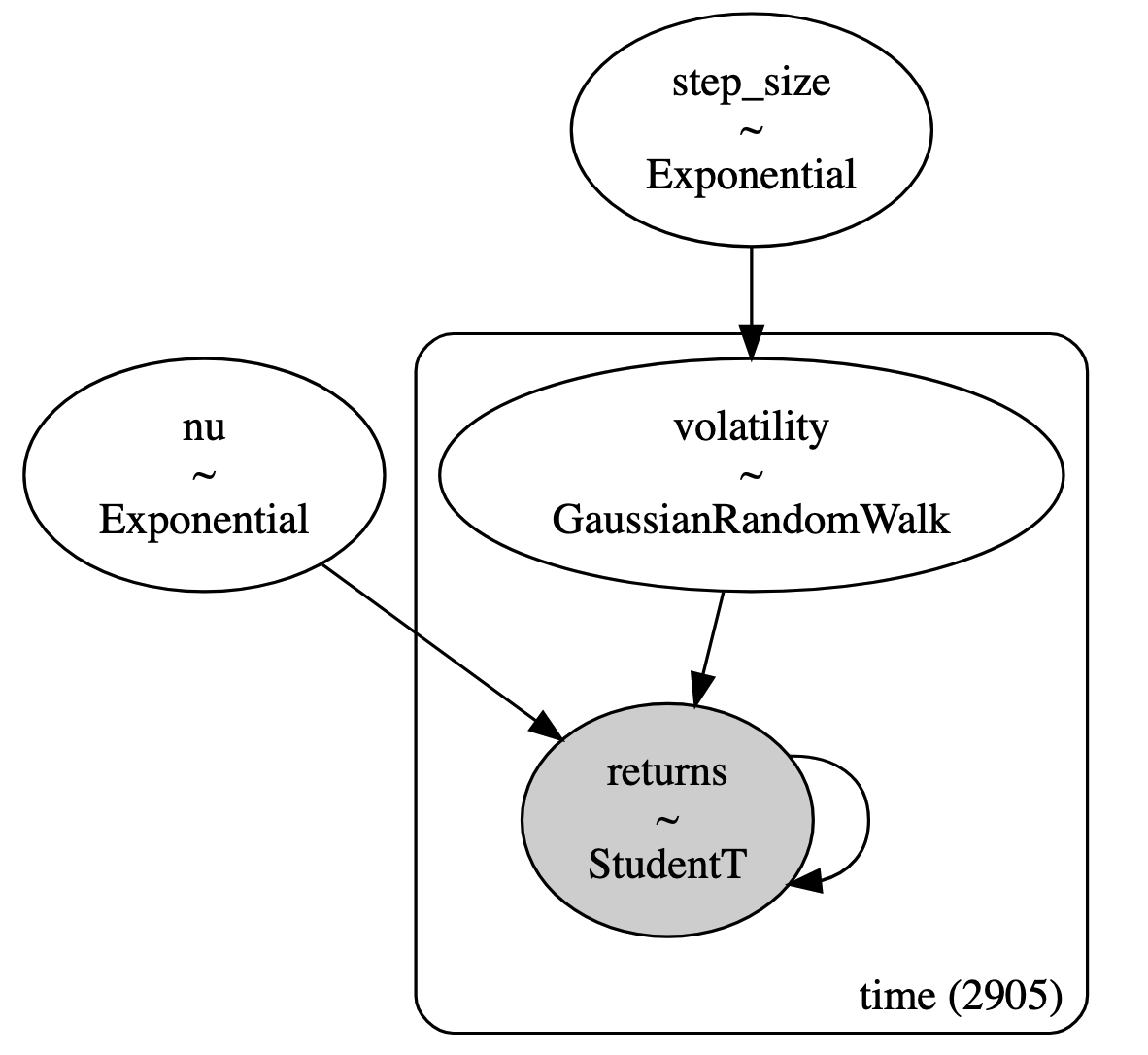
Figure 6: Stochastic volatility model described using plate notation ( source )
This is a relatively simple model for explaining asset prices. It is obviously too simple to actually model stock prices. One thing to point out is that we have a single variance (\(\sigma\)) for the volatility process across all time. This seems kind of unlikely given that we know different market regimes will behave quite differently. Further, I'm always pretty suspicious of Gaussian random walks. This implies some sort of stationarity, which obviously is not true over long periods of time (this may be an acceptable assumption at very short time periods though). In any case, it's a toy hierarchical model that we can use to test our two Bayesian learning methods.
5.2.1 Modelling the Hierarchy
The first thing to figure out is how to model Figure 6 using some combination of our two methods. Initially I naively tried applying SGLD directly but came across a major issue: how do I deal with the volatility term \(s_i\)? Naively applying SGLD means instantiating a parameter for each random variable you want to estimate uncertainty for, then applying SGLD using a standard gradient optimizer. Superficially, it looks very similar to using gradient descent to find a point estimate. The big problem with this approach is that the volatility \(s_i\) is conditional on the step size \(\sigma\). If we naively model \(s_i\) as a parameter, it loses its dependence on \(\sigma\) and are unable to represent the model in Figure 6.
It's not clear to me that there is a simple way around it using vanilla SGLD. The examples in [Welling2011] were non-hierarchical models such as Bayesian logistic regression that just needed to model uncertainty of the model coefficients. After racking my brain for a while on how to model it, I remembered that there was another example where one gets gradients to flow through a latent variable -- variational autoencoders! Yes, the good old reparameterization trick comes to save the day. This led me to the work on this generalization in [Blundell2015] and one of the ways you estimate uncertainty in Bayesian neural networks.
Let's write out some equations to make things more concrete. First the probability model with some simplifying notation of \(x_i = \log(r_i)\) for clarity:
Notice the random walk of the stochastic volatility \(s_i\) can be simplified by pulling out the mean, so we only have to worry about the additional zero-mean noise added at each step.
Why explicitly model \(s_i\) uncertainty at all?
One question you might ask is why do we need to explicitly model the uncertainty of \(s_i\) at all? Can't we just model \(\sigma\) (and \(\nu\)) and then apply SGLD, sampling the implied value of \(s_i\) along the way? Well it turns out that this doesn't quite work.
Naively for SGLD on the forward pass, you have a value for \(\sigma\), you can sample \(s_i = s_{i-1} + \sigma \cdot \varepsilon\) where \(\varepsilon \sim N(0, 1)\), then propagate and compute the associated t-distributed loss for \(x_i\). Similarly, you can easily backprop through this network since each computation is differentiable.
Unfortunately, this does not correctly capture the uncertainty specified in \(s_i\). One way to see this is that the sample we get using this method is \(s_i = s_0 + \sum_{i=1}^{i} \sigma \varepsilon\). This is just a random walk with standard deviation \(\sigma\) and starting point \(s_0\). Surely, the posterior of \(s_i\) is not just a scaled random walk. This would completely ignore the observed values of \(x_i\), which would only affect the value of \(\sigma\) (and \(\nu\)).
Another intuitive argument is that SGLD explores the uncertainty by "traversing" through the parameter space. Similar to more vanilla MCMC methods, it should spend more time in high density areas and less time in low density ones. If we are not "remembering" the values of \(s_i\) via parameters, then SGLD cannot correctly sample from the posterior distribution since it cannot "hang out" in high density regions of \(s_i\). That is why we need to both be able to properly model the uncertainty of \(s_i\) while still being able to backprop through it.
To deal with the hierarchical dependence of \(s_i\) on \(\sigma\), we approximate the posterior of \(s_i\) using a Gaussian with learnable mean \(\mu_i\) and \(\sigma\) as defined above:
Notice that \(q\) is not conditioned on \(\bf x\). In other words, we are going to use \(\bf x\) (via SGLD) to estimate the parameter \(\mu_i\), but there is no probabilistic dependence on \(\bf x\). Next using the ELBO from Equation 16, we want to be able to derive a loss to optimize our approximate posterior \(q(s_i|s_{i-1}, \sigma; \mu_i)\):
Finally, putting together our final loss based on the posterior we have:
We can see from Equation 39, that we have likelihood terms (\(\log p(x_i|s_i, \nu)\), \(\log p(s_i | s_{i-1}, \sigma)\)), prior terms (\(\log p(s_0)\), \(\log p(\sigma)\), \(\log p(\nu)\)), and a regularizer from our variational approximation (\(\log q(s_i|s_{i-1}, \sigma, \mu_i)\)). This is a common pattern in variational approximations with an ELBO loss.
With the loss we have enough to (approximately) model our stochastic volatility problem. First, start by defining a learnable parameter for each of \(\sigma, \nu, s_0, \mu_i\). Next, the forward pass is simply computing the \(s_i\) values using the reparameterization trick in Equation 37 using the loss from Equation 39. And with just the minor adjustments to make SGD into SGLD, you're off to the races!
An important point to make this practically train was to implement the RMSprop preconditioner from Equation 28. Without it I was unable to get a reasonable fit. This is probably analogous to most deep networks: if you don't use a modern optimizer, it's really difficult to fit a deep network. In this case we're modelling more than 2900 time steps, which can cause lots of issues when backpropagating.
5.2.2 Results
The first thing to look at are the results generated using HMC via PyMC, whose code was taken directly from the example. Figure 7 shows the posterior \(\sigma\) and \(\nu\) for two chains (two parallel runs of HMC). \(\sigma\) (step size) has a mode around 0.09 - 0.10 while \(\nu\) has a mode between 9 and 10. Recall that these variables parameterize an exponential distribution, so the expected value of the corresponding random variables are \(\sigma \approx 10\) and \(\nu \approx 0.1\) (the inverse of the parameter value).
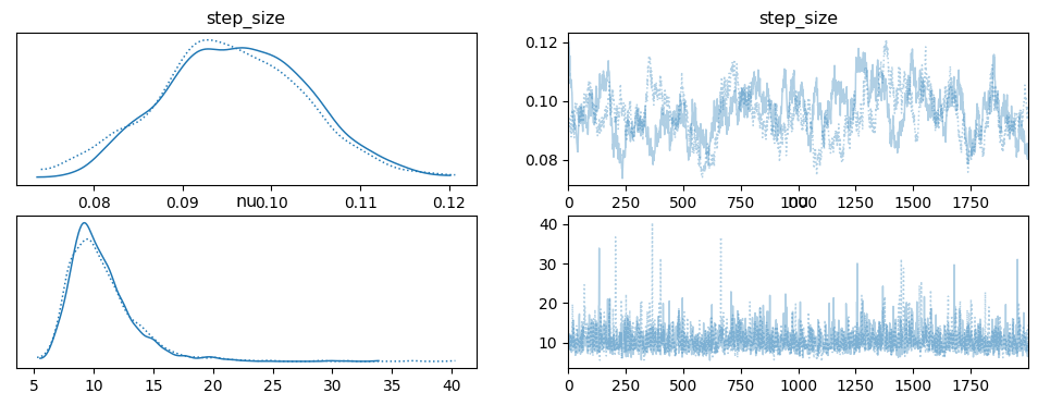
Figure 7: HMC posterior estimate of \(\sigma, \nu\) using PyMC
The more interesting distribution is the volatility shown in Figure 8. Here we see that there are certain times with high volatility such as 2008 (the financial crisis). These peaks in volatility also have higher uncertainty around them (measured by the vertical width of the graph), which matches our intuition that higher volatility usually means unpredictable markets making the volatility itself hard to estimate.
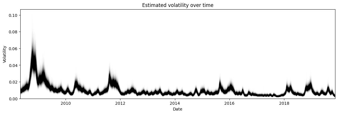
Figure 8: HMC posterior estimate of the volatility
The above stochastic volatility model was implemented using a simple PyTorch model Module and builtin the distributions package doing a lot of the heavy work. I used a mini-batch size of 100 by repeating the one trace 100 times. I found this stabilized the gradient estimates from the Gaussian sampled \(\bf s\) values. The RMSprop preconditioner was quite easy to implement by inheriting from the existing PyTorch class and overriding the \(step()\) function (see the notebook). I used a burnin of 500 samples with a fixed starting learning rate of 0.001 throughout the burnin after which the decayed polynomial learning rate schedule kicks in. I didn't use any thinning. Figure 9 shows the estimate for \(\sigma\) and \(\nu\) using SGLD.
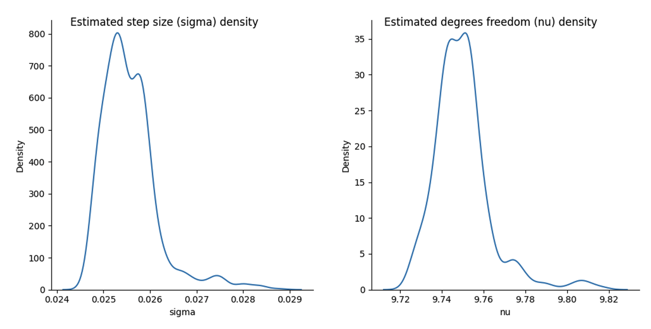
Figure 9: Posterior estimate of ** :math:`sigma, nu` **using SGLD
Starting with \(\nu\), its mode is not too far off with a value around \(9.75\), however the width of the distribution is much tighter with most of the density in between 9.7 and 9.8. Clearly either SGLD and/or our variational approximation has changed the estimate of the degrees of freedom.
This is even more pronounced with \(\sigma\). Here we get a mode around 0.025, which is quite different than the 0.09 - 0.10 we saw above with HMC. However, recall we are estimating parameters of a different model with \(\sigma\) is parameterizing the variance our approximate posterior, so we would expect that it wouldn't necessarily capture the same value. This points out a limitation of our approach: our parameter estimates in the approximate hierarchical model will not necessarily be comparable to the exact one. Thus, we don't necessarily get the interpretability of the model that we would expect in a regular Bayesian statistics flow.
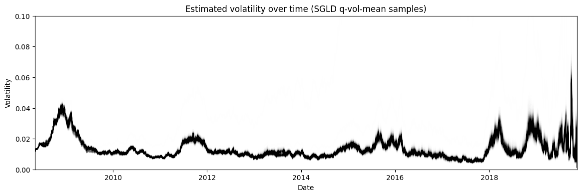
Figure 10: Posterior estimate of the stochastic volatility via SGLD of the approximate posterior mean
Finally, Figure 10 shows the posterior estimate of the stochastic volatility \(\bf s\). Recall, that we approximated \(s_i \approx q(\mu_i, \sigma) \sim N(\mu_i, \sigma)\). However, we cannot use \(q(\mu_i, \sigma)\) directly to estimate the volatility because that would mean the variance of the volatility at each timestep \(s_i\) would be equal, which clearly it is not. Instead, I used SGLD to estimate the distribution of each \(\mu_i\) and plotted that instead. Interestingly, we get a very similar shaped time series but with significantly less variance at each time step. For example, during 2008 the variance of the volatility hardly changes staying close to 0.04, whereas in the HMC estimate it's much bigger swinging from almost 0.035 to 0.08.
One reason that is often cited for the lower variance is that variational inference often underestimates the variance. This is because it is optimizing the KL divergence between the approximate posterior \(q\) and the exact one \(p\). This means that this is more likely to favour low variance estimates, see my previous post for more details. Another (perhaps more likely?) reason is that the approximation is just not a good one. Perhaps a more complex joint distribution across all \(s_i\) is what is really needed given the dependency between them. In any case, it points to the difficulty plugging these tools into a more typical Bayesian statistics workflow (which they were not at all intended to be used for by the way!).
5.3 Implementation Notes
Here are some unorganized notes about implementing the above two toy experiments. As usual, you can find the corresponding notebooks on Github.
In general, implementing SGLD is quite simple. Literally you just need to add a noise term to the gradient and update as usual in SGD. Just be careful that the variance of the Gaussian noise is equal to the learning rate (thus standard deviation is the square root of that).
The builtin distributions package in PyTorch is great. It's so much less error prone than writing out the log density yourself and it has so many nice helper functions like rsample() to do reparameterized sampling and log_prob() to compute the log probability.
The one thing that required some careful coding was adding mini-batches to the stochastic volatility model. It's nothing that complicated but you have to ensure all the dimensions line up and you are setting up your PyTorch distributions to have the correct dimension. Generally, you'll want one copy of the parameters but replicate them when you are computing forward/backward and then average over your batch size in your loss.
For computing the mixture distributions in the first experiment, I carelessly just took the weighted average of two Gaussians log densities -- this is not correct! The weighted average needs to be done in non-log space and then logged. Alternatively, it's just much easier to use the builtin PyTorch function of MixtureSameFamily() to do what you need.
One silly (but conceptually important) mistake was getting PyTorch scalars (i.e., zero dimensional tensors) and one dimensional tensors (i.e., vectors) with one element confused. Depending on the API, you're going to want one or the other and need to use squeeze() or unsqueeze() as appropriate.
Don't forget to use torch.no_grad() in your optimizer or else PyTorch will try to compute the computational graph of your gradient updates and cause an error.
For the brute force computation to estimate the exact posterior for the Gaussian mixture, you need to compute the unnormalized log density for a grid and the exponentiate it to get the probability. Obviously exponentiating it can cause overflow, so I scaled the unnormalized log density by subtracting the max value and then exponentiate. Got to pay attention to numerical stability sometimes!
For the stochastic volatility model for time step \(s_i\), the naive random walk posterior that we considered (by not modelling it at all) would cause the variance at \(Var(s_i) = \sum_{j=1}^i Var(s_j)\). This is because a random walk is a sum of independent random variables, meaning the sum at the \(i^{th}\) step is the sum of the variances. This is obviously not what we want.
I had to set the initial value of \(s_0\) close to the value of the posterior mean of \(s_1\) or else I didn't get something to fit well. I suspect that it's just really hard to backprop so far back and move the value of \(s_0\) significantly.
On that topic, I initialized \(\sigma, \nu\) to the means of the respective priors and \(\bf s\) to a small number near 0. Both of these seemed like reasonable choices.
I had to tune the number of batches in the stochastic volatility model to get a fit like you see above. Too little and it wouldn't get the right shape. Too much and it would get a strange shape as well with \(\sigma\) continually shrinking. I suspect the approximate Gaussian posterior is not really a good fit for this model.
While implementing the RMSprop preconditioner, I used inherited from the PyTorch implementation and overrode step() function. Using that function as a base, it's interesting to see all the various branches and special cases it handles beyond the vanilla one (e.g. momentum, centered, weighted_decay). Of course in my implementation I just ignored all of them and only implemented the simplest case but makes you appreciate the extra work that needs to be done to write a good library.
I added a random seed at some point in the middle just so I could reproduce my results. This was important because of the high randomness from the Bayes by Backprop sampling in the training. Obviously it's good practice but when you're just playing around it's easy to ignore.
6 Conclusion
Another post on an incredibly interesting topic. To be honest, I'm a bit disappointed that it wasn't some magical solution to doing Bayesian learning but it makes sense because otherwise all the popular libraries would have already implemented it. The real reason I got on this topic is because it is important conceptually to a stream of research that I've been trying to build up to. I find it incredibly satisfying to learn things "from the ground up", going back to the fundamentals. I feel that this is the best way to get a strong intuition for the techniques. The downside is that you go down so many rabbit holes and don't make too much direct progress towards a target. Fortunately, I'm not beholden to any sort of pressures like publishing so I can wander around to my heart's desire. As they say, it's about the journey not the destination. See you next time!
7 References
Previous posts: Markov Chain Monte Carlo and the Metropolis Hastings Algorithm, Hamiltonian Monte Carlo, The Expectation Maximization Algorithm, Variational Autoencoders, An Introduction to Stochastic Calculus
- Welling2011(1,2,3,4)
-
Max Welling and Yee Whye Teh, "Bayesian Learning via Stochastic Gradient Langevin Dynamics", ICML 2011.
- Blundell2015(1,2,3,4,5)
-
Blundell et. al, "Weight Uncertainty in Neural Networks", ICML 2015.
- Li2016(1,2,3)
-
Li et. al, "Preconditioned Stochastic Gradient Langevin Dynamics for Deep Neural Networks", AAAI 2016.
- Radford2012(1,2)
-
Radford M. Neal, "MCMC Using Hamiltonian dynamics", arXiv:1206.1901, 2012.
- Teh2015(1,2,3,4,5,6)
-
Teh et. al, "Consistency and fluctations for stochastic gradient Langevin dynamics", arXiv:1409.0578, 2015.
- Dauphin2015(1,2)
-
Dauphin et. al, "Equilibrated adaptive learning rates for non-convex optimization", arXiv:1502.04390, 2015.