Hamiltonian Monte Carlo
Here's a topic I thought that I would never get around to learning because it was "too hard". When I first started learning about Bayesian methods, I knew enough that I should learn a thing or two about MCMC since that's the backbone of most Bayesian analysis; so I learned something about it (see my previous post). But I didn't dare attempt to learn about the infamous Hamiltonian Monte Carlo (HMC). Even though it is among the standard algorithms used in Bayesian inference, it always seemed too daunting because it required "advanced physics" to understand. As usual, things only seem hard because you don't know them yet. After having some time to digest MCMC methods, getting comfortable learning more maths (see here, here, and here), all of a sudden learning "advanced physics" didn't seem so tough (but there sure was a lot of background needed)!
This post is the culmination of many different rabbit holes (many much deeper than I needed to go) where I'm going to attempt to explain HMC in simple and intuitive terms to a satisfactory degree (that's the tag line of this blog after all). I'm going to begin by briefly motivating the topic by reviewing MCMC and the Metropolis-Hastings algorithm then move on to explaining Hamiltonian dynamics (i.e., the "advanced physics"), and finally discuss the HMC algorithm along with some toy experiments I put together. Most of the material is based on [1] and [2], which I've found to be great sources for their respective areas.
Table of Contents
1 Background
1.1 Markov Chain Monte Carlo
This section is going to give a brief overview of MCMC and the Metropolis-Hastings algorithm. For a more detailed treatment, see my previous post.
Markov Chain Monte Carlo (MCMC) algorithms are a class of techniques that use Markov chains to sample from a target probability distribution ("Monte Carlo"). The main idea is that you construct a Markov Chain such that the steady state distribution of the Markov Chain approximates your target distribution. The samples from your target distribution can then be generated just by traversing that Markov Chain.
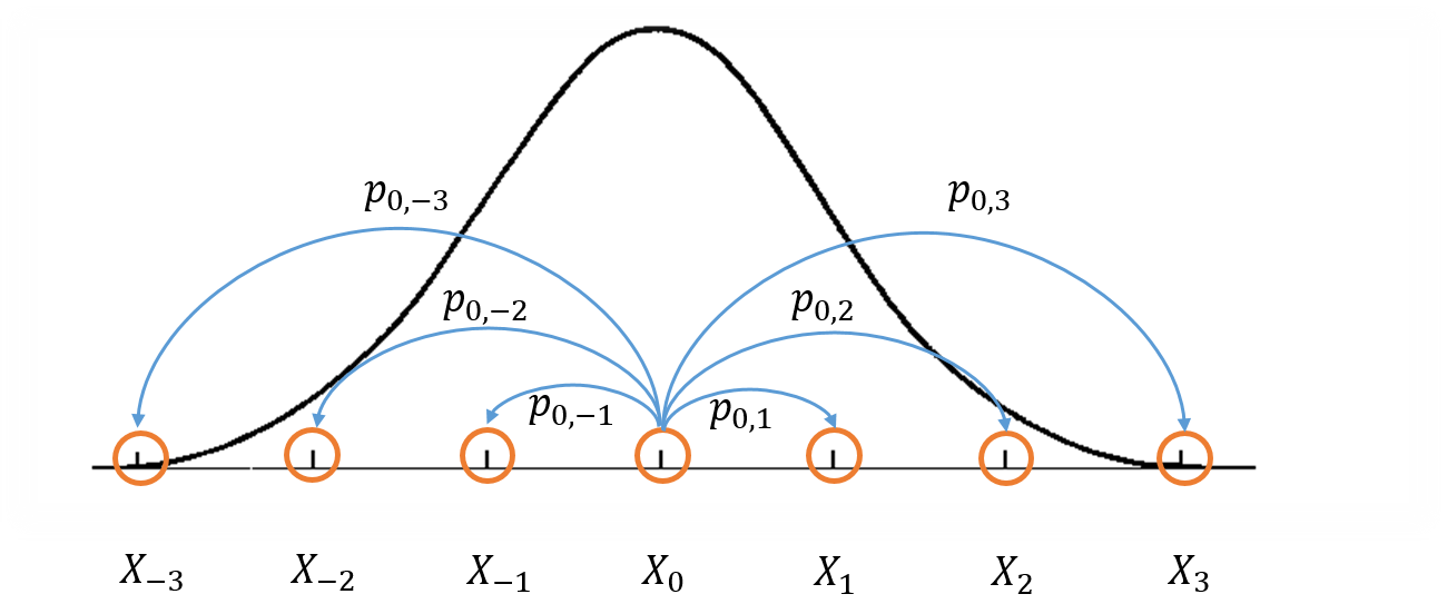
Figure 1: Visualization of a Markov Chain Monte Carlo.
Figure 1 shows a crude visualization of the idea. The "states" of the Markov Chain are the support of your probability distribution (the figure only shows states with discrete values for simplicity but they can also be continuous). Three important conditions that are required to construct a Markov chain that can be used for MCMC are:
Irreducible: We must be able to reach any one state from any other state eventually (i.e. the expected number of steps is finite).
Aperiodic: The system never returns to the same state with a fixed period.
Reversible (aka Detailed Balance): A Markov chain is called reversible if the Markov chain has a stationary distribution \(\pi\) such that \(\pi_i T(i|j) = \pi_j T(j|i)\) where \(T(i|j)\) is the transition probability from state \(i\) to \(j\) and \(\pi_i\) and \(\pi_j\) are the equilibrium probabilities for their respective states. This condition is known as the detailed balance condition.
The first two properties define a Markov chain which is ergodic, which implies that there is a steady state distribution. The third property is used to ensure that the Markov chain can be used in an MCMC algorithm.
One of the earliest MCMC algorithms was the Metropolis-Hastings algorithm (see my previous post for a derivation). This algorithm is nice because you don't need the actual probability density, call it \(p(x)\), but rather only a function that is proportional to it (\(f(x) \propto p(x)\)). Assuming that the state space of the Markov Chain is the support of your target probability distribution, the algorithm gives a method to select the next state to traverse. It does this by introducing two new distributions: a proposal distribution \(g(x)\) and an acceptance distribution \(A(x)\). The proposal distribution only needs to have the same support as your target distribution, although it's much more efficient if it has a similar shape. The acceptance distribution is defined as:
with \(y\) being the newly proposed state sampled from your proposal distribution \(g(x)\). The \(y | x\) notation means that the proposal distribution is conditioned on the current state (\(x\)) with a proposed transition to the next state (\(y\)). The idea is that the proposal distribution will change depending on the current state. A common choice is a normal distribution centered on \(x\) with a standard deviation dependent on the problem instance.
The algorithm can be summarized as such:
Initialize the initial state by picking a random \(x\).
Propose a new state \(y\) according to \(g(y | x)\).
Accept state \(y\) with uniform probability according to \(A(y | x)\). If accepted transition to state \(y\), otherwise stay in state \(x\).
Go to step 2 (repeat \(T\) times).
Save the current state as a sample, repeat steps 2-4 to sample another point.
Notice that in step 4 we throw away a bunch of samples before we return one in step 5. This is because sequential samples will be typically be correlated, which is the opposite of what we want. So we throw away a bunch of samples in hopes that the sample we pick is sufficiently independent. Theoretically, as we approach an infinite number of samples this doesn't make a difference, but practically we need it in order to generate random independent samples with a finite run.
To make MH efficient, you want your proposal distribution to accept with a high probability (so that you can make \(T\) small), otherwise you get stuck in the same state and it takes a very long time for the algorithm to converge. This means you want \(g(y|x) \approx f(y)\). If they are approximately equal, then the fraction in Equation 1 is approximately 1 ensuring the acceptance rate (step 3) is relatively high, but this isn't so easy to do. If we had a closed form for the density then we could just sample from the original distribution directly, which would negate the need for MCMC in the first place! Fortunately, there are other algorithms like HMC that can do better (in most cases).
1.2 Motivation
Let's take a look at the basic case of using a normal distribution as our proposal distribution centered on our current state (in 1D). We can see that \(g(x | y) = g(y | x)\) making our proposal symmetric. In other words, the probability of jumping from \(x\) to \(y\) is equal to the probability of jumping from \(y\) to \(x\). So the fraction in Equation 1 then becomes simply \(\frac{f(y)}{f(x)}\). This implies that you're more than likely to stick around in state \(x\) if it has a high density, and unlikely to move to state \(y\) if it has low density, which matches our intuition of what should happen.
This method is typically called "random walk" Metropolis-Hastings because you're randomly selecting a point from your current location. It works well in some situations but it's not without its problems. The main issue is that it doesn't very efficiently explore the state space. Figure 2 shows a visualization of this idea.
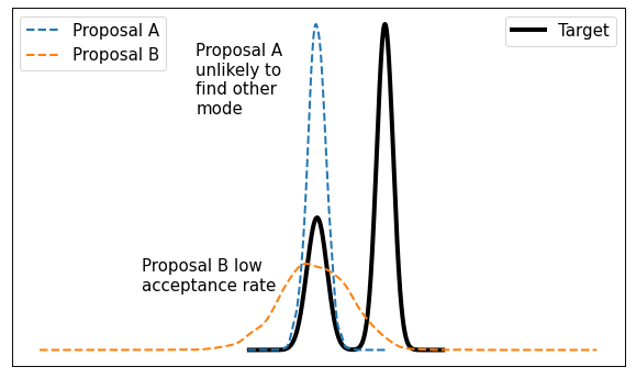
Figure 2: It's difficult to calibrate random walk MH algorithms
From Figure 2, consider a bimodal distribution with a random walk MH algorithm. If you start in one of the modes (left side) with a very tight proposal distribution (Proposal A), you may get "stuck" in that mode without visiting the other mode. Theoretically, you'll eventually end up in the other mode but practically you might not get there with a finite MCMC run. On the other hand, if you make the variance large (Proposal B) then in many cases you'll end up proposing states where \(f(y)\) is small, making the acceptance rate from Equation 1 small. There's no easy way around it, there will always be this sort of trade-off and it's only exacerbated in higher dimensions.
However, we've just been talking about random walk proposal distributions. What if there was a better way? Perhaps one where you can (theoretically) get close to a 100% acceptance rate? How about one where you don't need to throw away any samples (Step 4 from MH algorithm above)? Sounds too good to be true doesn't it? Yes, yes it is too good to be true, but we can sort of get there with Hamiltonian Monte Carlo! But let's not get ahead of ourselves, let's first start with an explanation of Hamiltonian Dynamics.
2 Hamiltonian Mechanics
Before we dive into Hamiltonian dynamics, let's do a quick review of high school physics with Newton's second law of motion to understand how we can use it to describe the motion of (macroscopic) objects. Then we'll move on to a more abstract method of describing these systems with Lagrangian mechanics. Finally, we'll move on to Hamiltonian mechanics (and its approximations), which can be considered as a modification of Lagrangian mechanics. We'll see that these concepts are not as scary as they sound, as long as we remember some calculus and how to solve some relatively simple differential equations.
2.1 Classical Mechanics
Classical mechanics (or Newtonian mechanics) is the physical theory that describes the motion of macroscopic objects like a ball, spaceship or even planetary bodies. I won't go much into detail on classical mechanics and assume you are familiar with the basic concepts from a first course in physics.
One of the main tools we use to describe motion in classical mechanics is Newton's second law of motion:
Where \(\bf F_{net}\) is the net force on an object, \(m\) is the mass of the object, \(\bf a(t)\) is the acceleration, \(\bf x(t)\) is the position (with respect a reference), and bold quantities are vectors.
Notice that Equation 2 is a differential equation, where \(\bf x(t)\) describes the equation of motion of the object over time. In high school physics you may not have had to solve differential equations. Instead, you may have been given equations to solve for \(x(t)\) assuming a constant acceleration. Now that we know better though, we can remove that simplification and write things in terms of differential equations.
Note that I use the notation \(x'(t) := \frac{dx}{dt}\) to always represent the time derivative of the function \(x(t)\) (or later on \(p\) and \(q\)). Most physics sources use the "dot" (\(\dot{x}(t)\)) notation to represent time derivatives but I'll use the apostrophe because I think it's probably more familiar to non-physics readers.
I won't spend too much more time on this except to give a running example that we'll use throughout the rest of this section.
Example 1: A Simple Harmonic Oscillator using classical mechanics.
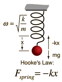
Figure 3: Simple Harmonic Oscillator (source: [3])
Consider a mass (\(m\)) suspended from a spring in Figure 3, where \(k\) is the force constant of the spring, and positive \(x\) is the downward direction with \(x=0\) set at the spring's equilibrium. Using Newton's second law (Equation 2), we get the following differential equation (where acceleration is the second time derivative of position):
Rearranging:
Here we are defining a new function \(y(t)\) that is shifted by \(x_0\). This is basically the same as defining a new coordinate system shifted by \(x_0\) from our original one. Notice that \(\frac{d^2 y(t)}{dt^2} = \frac{d^2 x(t)}{dt^2}\) since the constant vanishes with the derivative. And so we end up with the simplified differential equation:
In this case, it's a second order differential equation with complex roots. I'll spare you solving it from scratch and just point you to this excellent set of notes by Paul Dawkins. However, we can also just see by inspection that a solution is:
Given an initial position and velocity, we can solve Equation 6 for the particular constants.
Example 1 gives the general idea of how to find the motion of an object:
Calculate the net forces.
Solve the (typically second order) differential equation from Equation 2 (Newton's second law).
Apply initial conditions (usually position and velocity) to find the constants.
It turns out this is not the only way to find the equation(s) of motion. The next section gives us an alternative that is sometimes more convenient to use.
2.2 Lagrangian Mechanics
Instead of using the classical formulation to solve the equation, we can use the Lagrangian method. It starts out by defining this strange quantity called the Lagrangian 1:
Where the Lagrangian is (typically) a function of the position \(x(t)\), its velocity \(\frac{dx(t)}{dt}\), and time \(t\). It is kind of strange that we have a minus sign here and not a plus (which would give the total energy) but it turns out that's what we want here. We're going to show that we can use the Lagrangian to arrive at the same mathematical statement as Newton's second law by way of a different method. It's going to be a bit round about but we'll go through several useful mathematical tools along the way (which will eventually lead us to the Hamiltonian).
We'll start off by defining what is called the action that uses the Lagrangian:
The astute reader will notice that Equation 8 is a functional. Moreover, it's precisely the functional defined by the Euler-Lagrange equation. For those who have not studied this topic, I'll give a brief overview here but direct you to my blog post on the calculus of variations for more details.
Equation 8 is what is called a functional: a function \(S[x(t)]\) of a function \(x(t)\), where we use the square bracket to indicate a functional. That is, if you plug in a function \(x_1(t)\) you get a scalar out \(S[x_1(t)]\); if you plug in another function \(x_2(t)\), you get another scalar out \(S[x_2(t)]\). It's a mapping from functions to scalars (as opposed to scalars to scalars).
Equation 8 depends only on the function \(x(t)\) (and it's derivative) since \(t\) gets integrated out. Functionals have a lot of similarities to the traditional functions we are used to in calculus, in particular they have the analogous concept of derivatives called functional derivatives (denoted by \(\frac{\delta S}{\delta x}\)). One simple way to compute the functional derivative is to use the Euler-Lagrange equation:
Here I'm dropping the parameters of \(L\) and \(x\) to make things a bit more readable. Equation 9 can be computed using our usual rules of calculus since \(L\) is just a multivariate function of \(t\) (and not a functional). The proof of Equation 9 is pretty interesting but I'll refer you to Chapter 6 of [2] if you're interested (which you can find online as a sample chapter).
Historical Remark
As with a lot of mathematics, the Euler-Lagrange equation has its roots in physics. A young Lagrange at the age of 19 (!) solved the tautochrone problem in 1755 developing many of the mathematical ideas described here. He later sent it to Euler and they both developed the ideas further which led to Lagrangian mechanics. Euler saw the potential in Lagrange's work and realized that the method could extend beyond mechanics, so he worked with Lagrange to generalize it to apply to any functionals of that form, developing variational calculus in the process.
So why did we introduce all of these seemingly random expressions? It turns out that they are useful in the principle of least action:
The path taken by the system between times \(t_1\) and \(t_2\) and configurations \(x_1\) and \(x_2\) is the one for which the action is stationary (i.e. no change) to first order.
where \(t_1\) and \(t_2\) are the initial and final times, and \(x_1\) and \(x_2\) are the initial and final position. It's sounds fancy but what it's saying is that if you find a stationary function of Equation 8 (where the first functional derivative is zero) then it describes the motion of an object. The derivation of it relies on quantum mechanics, which is beyond the scope of this post (and my investigation on the subject).
However, if the principle of least action describes the motion then it should be equivalent to the classical mechanics approach from the previous subsection -- and it indeed is equivalent! We'll show this in the simple 1D case but it works in multiple dimensions and with different coordinate bases as well. Starting with a general Lagrangian (Equation 7) for an object:
Here we're using the standard kinetic energy formula (\(K=\frac{1}{2}mv^2\), where velocity \(v=x'(t)\)) and a generalized potential function \(U(x(t))\) that depends on the object's position (e.g. gravity). Plugging \(L\) into the Euler-Lagrange (Equation 9) and setting it to zero to find the stationary point, we get:
So we can see that we end up with Newton's second law of motion as we expected. The negative sign comes in because if we decrease the potential (change in potential is negative), we're moving in the direction of the potential field, thus we have a positive force.
So we went through all of that to derive the same equation? Pretty much, but in certain cases the Lagrangian is easier to formulate and solve than the classical approach (although not in the simple example below). Additionally, it is going to be useful to help us derive the Hamiltonian.
Example 2: A Simple Harmonic Oscillator using Lagrangian mechanics.
Using the same problem in Example 1, let's solve it using the Lagrangian. We can define the Lagrangian as (omitting the parameters for cleanliness):
where each term represents the velocity, gravitational potential and elastic potential of the spring respectively. Recall \(x=0\) is defined to be where the spring is at rest and positive \(x\) is the downward direction. Thus, the gravitational potential is negative of the \(x\) direction while the spring has potential with any deviation from \(x=0\).
Using the Euler-Lagrange equation (and setting it to 0):
And we see we end up with the same second order differential equation as Equation 4, which yields the same solution \(x(t) = Acos(\frac{k}{m}t + \phi)\). We didn't really gain anything by using the Lagrangian but often times in multiple dimensions, potentially with a different coordinate basis, the Lagrangian method is easier to use.
One last note before we move on to the next section. It turns out the Euler-Lagrange equation from Equation 9 is agnostic to the coordinate system we are using. In other words, for another coordinate system \(q_i:= q_i(x_1,\ldots,x_N;t)\) (with the appropriate inverse mapping \(x_i:= x_i(q_1,\ldots,q_N;t)\)), the Euler-Lagrange equation still works:
From here on out instead of assuming Cartesian coordinates (denoted with \(x\)'s), we'll be using the generic \(q\) to denote position with its corresponding first (\(q'\)) and second derivatives (\(q''\)) for velocity and acceleration, respectively.
2.3 The Hamiltonian and Hamilton's Equations
We're slowly making our way towards HMC and we're almost there! Let's discuss how we can solve the equations of motion using Hamiltonian mechanics. We first start off with another esoteric quantity:
where we have potentially \(N\) particles and/or coordinates. The symbol \(E\) is used because usually Equation 15 is the total energy of the system. Let's show that in 1D using the fact that \(L=K-U=\frac{1}{2}mq'^2 - U(q)\) for potential energy \(U(q)\):
where we can see that it's the kinetic energy plus the potential energy of the system. If the coordinate system you are using is Cartesian, then it is always the total energy. Otherwise, you have to ensure the change of basis does not have a time dependence or else there's no guarantee. See 15.1 from [2] for more details.
Now we're almost at the Hamiltonian with Equation 15 but we want to do a variable substitution by getting rid of \(q'\) and replacing it with something called the generalized momentum (to match our generalized position \(q\)):
This is sometimes the same as the usual linear momentum (usually denoted by \(p\)) you learn about in a first physics class. Assuming we have the usual equation for kinetic energy with Cartesian coordinates:
However, for example, if you are dealing with angular kinetic energy (such as a swinging pendulum) and using those coordinates, then you'll end up with angular momentum instead. In any case, all we need to know is Equation 17. Substituting it into our (often) total energy equation (Equation 15) and re-writing in terms of only \(q\) and \(p\) (no explicit \(q'\)), we get the Hamiltonian:
where I've used bold to indicate vector quantities. Notice that we didn't explicitly eliminate \(q'_i\), we just wrote it as a function of \(q\) and \(p\).
The \(2n\) dimensional coordinates \(({\bf q, p})\) are called the phase space coordinates (also known as canonical coordinates). Intuitively, we can just think of this as the position (\(x\)) and linear momentum (\(mv = mx'\)), which is what you would expect if you were asked for the current state of a system (alternatively you could use velocity instead of momentum). However, as we'll see later, phase space coordinates have certain nice properties that we'll utilize when trying to perform MCMC.
Now Equation 19 by itself maybe isn't that interesting, but let's see what happens when we analyze how it changes with respect to its inputs \(q\) and \(p\) (in 1D to keep things cleaner). Starting with \(p\):
Now isn't that nice? The partial derivative with respect to the generalized momentum of the Hamiltonian simplifies to the velocity. Let's see what happens when we take it with respect to the position \(q\):
Similarly, we get a (sort of) symmetrical result where the partial derivative with respect to the position is the negative first time derivative of the generalized momentum. Equations 20 and 21 are called Hamilton's equations, which will allow us to compute the equation of motion as we did in the previous two methods. The next example shows this in more detail.
Explanation of \(\frac{\partial L(q, q'(q, p))}{\partial q} = \frac{\partial L(q, q')}{\partial q} + \frac{\partial L(q, q')}{\partial q'} \frac{\partial q'(q, p)}{\partial q}\)
This expression is partially (get it?) confusing because of the notation and partially confusing because it's not typically seen when discussing the chain rule for partial differentiation. Notice that the LHS looks almost identical to the first term in the RHS. The difference being that \(q'(q, p)\) is a function of \(q\) on the LHS, while on the RHS it's constant with respect to \(q\). To see that, let's re-write the LHS using some dummy functions.
Define \(f(q) = q\) and \(g(q, p) = q'(q, p)\), and then substitute into the LHS and apply the chain rule for partial differentiation:
As you can see the first term on the RHS has a "constant" \(q'\) from the partial differentiation of \(f(q) = q\). The notation seems a bit messy, I did a double take when I first saw it, but hopefully this makes it clear as mud.
Example 3: A Simple Harmonic Oscillator using Hamiltonian mechanics.
Using the same problem in Example 1 and 2, let's solve it using Hamiltonian mechanics. We start by writing the Lagrangian (repeating Equation 12):
Next, calculate the generalized momentum (Equation 17):
Which turns out to just be the linear momentum. Note, we'll be using \(x\) instead of \(q\) in this example since we'll be using standard Cartesian coordinates.
From Equation 23, solve for the velocities (\(x'\)) so we can re-write in terms of momentum, we get:
Write down the Hamiltonian (Equation 19) in terms of its phase space coordinates \((x, p)\), eliminating all velocities using Equation 24:
Write down Hamilton's equation (Equation 20 and 21):
Finally, we just need to solve these differential equations for \(x(t)\). In general, this involves eliminating \(p\) in favor of \(x'\). In this case it's quite simple. Notice that Equation 26 is exactly Newton's second law (where \(\frac{dp}{dt} = m\frac{dx'}{dt} = ma\)) and mirrors Equation 3, while Equation 27 is just the definition of velocity (where \(p=mv\)). As a result, we'll end up with exactly the same solution for \(x(t)\) as the previous examples.
2.4 Properties of Hamiltonian Mechanics
After going through example 3, you may wonder what was the point of all of this manipulation? We essentially just ended with Newton's second law, which required an even more round about way via writing the Lagrangian, Hamiltonian, Hamilton's equations and then converting it back to where we started. These are all very good observations and the simple examples shown so far don't do Hamiltonian mechanics justice. We usually do not use the Hamiltonian method for standard mechanics problems involving a small number of particles. It really starts to shine when using it for analyses with a large number of particles (e.g. thermodynamics) or with no particles at all (e.g. quantum mechanics where everything is a wave function). We won't get into these two applications because they are beyond the scope of this post.
However, another nice thing about the Hamiltonian form is that it has nice some properties that aren't obvious at first glance. There are three properties that we'll care about:
Reversability: For a particle, given its initial point in phase space \((q_0, p_0)\) at a point in time, its motion is completely (and uniquely) determined for all time. That is, we can use Hamilton's equations to find its instantaneous rate of change (\((q', p')\)), which can be used to find its nearby position after a delta of time, and repeated to find its complete trajectory. This hints at the application we're going to use it for: using a numerical method to find its trajectory (next subsection). Equally important though is the fact that we can reverse this process to find where it came from. If you have a path from \((q(t), p(t))\) to \((q(t+s), p(t+s)\) then you can reverse the operation by negating its time derivative (\((-q', -p')\)) and move backwards along its trajectory. This is because each trajectory is unique in phase space. We'll use this property when constructing the Markov chain transitions for HMC.
Conservation of the Hamiltonian: Another important property is that the Hamiltonian is conserved. We can see this by taking the time derivative of the Hamiltonian (in 1D to keep things simple):
This important property lets us almost get to a 100% acceptance rate for HMC. We'll see later that this ideal is not always maintained.
Volume preservation: The last important property we'll use it called Liouville's theorem (from [2]):
Liouville's Theorem: Given a system of \(N\) coordinates \(q_i\), the \(2N\) dimensional "volume" enclosed by a given \((2N-1)\) dimensional "surface" in phase space is conserved (that is, independent of time) as the surface moves through phase space.
I'll refer to [2] if you want to see the proof. This is an important result that will be used to avoid accounting for the change in volume (via Jacobians) in our HMC algorithm since the multi-dimensional "volume" is preserved. More on this later.
2.5 Discretizing Hamiltonian's Equations
The simple examples we saw in the last subsections worked out nicely because we could solve the differential equations for a closed form solution. As you can imagine in most cases, we won't have such a nice closed form solution. Thus, we turn to approximate methods to compute our desired result (the equations of motion).
One way to approach it is to iteratively simulate Hamilton's equation by discretizing time using some small \(\epsilon\). Starting at time 0, we can iteratively compute the trajectory in phase space \((q, p)\) through time using Hamilton's equations. We'll look at two and a half methods to accomplish this.
Euler's Method: Euler's method is a technique to solve first order differential equations. Notice that Hamilton's equations produce 2N first order differential equations (as opposed to the Lagrangian, which produces second order differential equations). Euler's method works by applying a first order Taylor series approximation at each iteration about the current point.
More precisely, for a given step size \(\epsilon\), we can approximate the curve \(y(t)\) given an initial point \(y_0\) and a first order differential equation using the formula:
where \(y(t_0)=y_0\) and \(y'(t, y(t))\) is our first order differential equation. This method simply takes small step sizes along the gradient of our curve where the gradient is computed from our differential equation using \(t\) and the previous values of y.
Translating this to phase space and using Hamilton's equations, we have:
Notice that the equations are dependent on each other, to calculate \(p(t+\epsilon)\) or \(q(t+\epsilon)\), we need both \((q(t), p(t))\).
The main problem with Euler's method is that it quickly diverges from the actual curve because of the accumulation of errors. The error propagates because we assume we start from somewhere on the curve, whereas we're always some delta away from the curve after the first iteration. Figure 4 (top left) shows how the method quickly spirals out of control towards infinity even with a small epsilon with our simple harmonic oscillator from Examples 1-3 (the black line shows the exact trajectory).
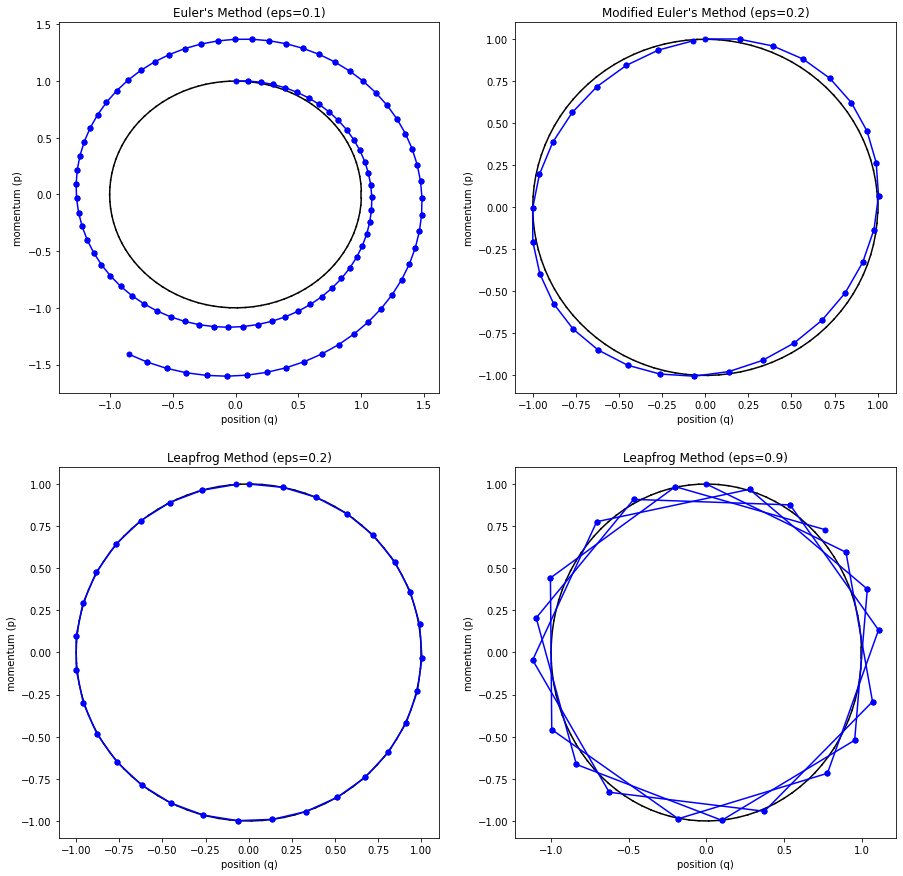
Figure 4: Methods to approximate Hamiltonian dynamics: Euler's method, modified Euler's method, and Leapfrog using the harmonic oscillator from Examples 1-3.
Modified Euler's Method: A simple modification to Euler's method is to update \(p\) and \(q\) separately. First update \(p\), then use that result to update \(q\) and repeat (the other way around also works). More precisely, we get this approximation in phase space:
The results can be seen in Figure 4 (top right) where it much more closely tracks the underlying curve without tendencies to diverge.
This reason for this is because the pair of equations preserves volume just like the result from Liouville's theorem above. Let's show how that is the case in two dimensions but this result also holds for multiple dimensions. (In fact, a similar idea used in the following argument can be used to prove Liouville's theorem.)
First note that Equation 31 can be viewed as a transformation mapping \((p(t), q(t))\) to \((p(t+\epsilon), q(t))\) (same for Equation 32). Denote this mapping as \(\bf f\) and let's analyze how the differentials of the above equation change. Note: I'll change all the parameters to superscripts to make the notation a bit cleaner. First, we can see the transformation for Equation 31 as:
Next, let's calculate the Jacobian of \(\bf f\):
We can clearly see the determinant of the Jacobian is 1. Next let's see how the infinitesimal volume (or area in this case) changes using the substitution rule (this is usually not shown since having a unit Jacobian determinant already implies this):
So we see that the volume is preserved when we take an arbitrarily small step (Equation 31). We can use the same logic for Equation 32 and thus every subsequent application of those equations also preserves volume.
Figure 5 shows this visually by drawing a small region near the starting points and then running Euler's method and modified Euler's method. For the vanilla Euler's method, you can see the region growing larger with each iteration. This has the tendency to cause points to spiral out to infinity (since the area of this region grows, so do the points that define it). Modified Euler's doesn't have this problem.
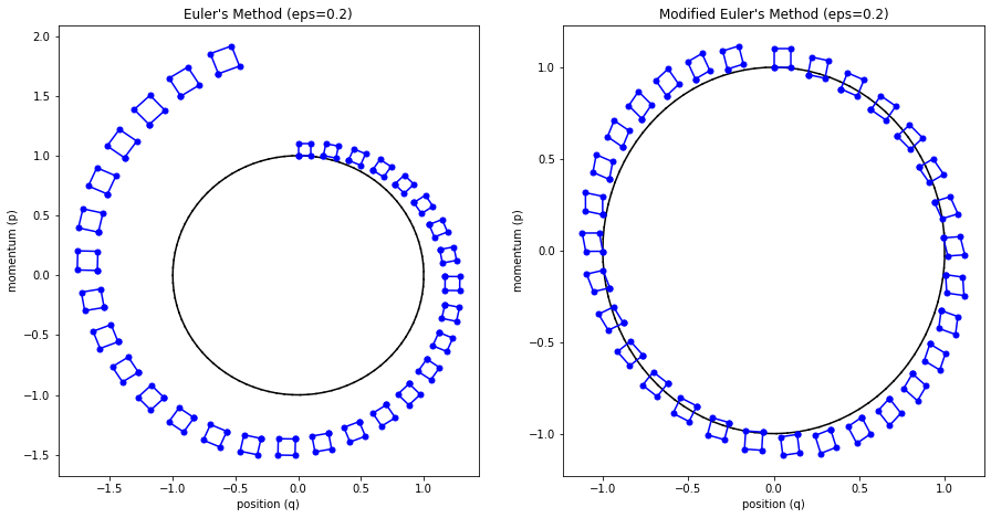
Figure 5: Contrasting volume preservation nature of the modified Euler's method vs. Euler's method.
It's not clear to me that volume preservation in general guarantees that it won't spiral to infinite, nor that non-volume preservation necessarily guarantees it will spiral to infinite but it does sure seem to help empirically. The guarantees (if any) are likely related to the symplectic nature of the method but I didn't really look into it much further than that.
Leapfrog Method: The final method uses the same idea but with an extra Leapfrog step:
where we iteratively apply these equations in sequence similar to modified Euler's method. The idea is that instead of taking a "full step" for \(p\), we take a "half step" (Equation 35). This half step is used to update \(q\) with a full step (Equation 36), which is then used to update \(p\) using another "half step" (Equation 37). The last two subplots (bottom left and right) in Figure 4 show Leapfrog in action, which empirically performs much better than the other methods.
Using the same logic as above, each transform individually is volume preserving, ensuring similar "nice" behaviour as modified Euler's method. Notice we're doing slightly more "work" in that we're evaluating Hamilton's equations an additional time but the trade-off is good in this case.
Another nice property of both modified Euler's and Leapfrog is that it is also reversible. Simply negate \(p\), and run the algorithm, then negate \(p\) to get back where you started. This works because the momentum is the only thing causing motion, so negating \(p\) essentially reverses our direction. Since we're only updating either \(p\) or \(q\), it allows us to essentially run the algorithm in reverse. As you might guess, this reversibility condition is going to be helpful for use in MCMC.
3 Hamiltonian Monte Carlo
Finally we get to the good stuff: Hamiltonian Monte Carlo (HMC)! The main idea behind HMC is that we're going to use Hamiltonian dynamics to simulate moving around our target distribution's density. The analogy used in [1] is imagine a puck moving along a frictionless 2D surface 2. It slides up and down hills, losing or gaining velocity (i.e. kinetic energy) based on the gradient of the hill (i.e. potential energy). Sound familiar? This analogy with a physical system is precisely the reason why Hamiltonian dynamics is such a good fit.
The mapping from the physical situation to our MCMC procedure will be such that the variables in our target distribution will correspond to the position (\(q\)), the potential energy will be the negative log probability density of our target distribution, and the momentum variables (\(p\)) will be artificially introduced to allow us to sample properly. So without further adieu, let's get into the details!
3.1 From Thermodynamics to HMC
The physical system we're going to base this on is from thermodynamics (which is only slightly more complex than the mechanical systems we're been looking at). A commonly studied situation in thermodynamics is one of a closed system of fixed volume and number of particles (e.g. gas molecules in a box) that is "submerged" in a heat bath at thermal equilibrium. The idea is the heat bath is much, much larger than our internal system so it can keep it the system at a constant temperature. Note that even though internal system is at a constant temperature, its energy will fluctuate because of the mechanical contact with the heat bath, so the internal system energy is not conserved (i.e., constant). The overall energy of the combined system (heat bath and internal system) is conserved though. This setup is called the canonical ensemble.
One of the fundamental concepts in thermodynamics is the idea of a microstate, which defines (for classical systems) a single point in phase space. That is, the position (\(q\)) and momentum (\(p\)) variables for all particles defines the microstate of the entire system. In thermodynamics, we are typically not interested in the detailed movement of each particle (although will be for MCMC), instead usually want to measure other macro thermodynamic quantities such as average energy or pressure of the internal system.
An important quantity we need to compute is the probability of the internal system being in a particular microstate i.e., a given configuration of \(p\)'s and \(q\)'s. Without going into the entire derivation, which would take us on a larger tangent into thermodynamics, I'll just give the result, which is known as the Boltzman distribution:
where \(p_i\) is the probability of being in state \(i\), \(P(q, p)\) is the same probability but explicitly labelling the state with its phase state coordinates \((q, p)\), \(E_i\) is the energy state of state \(i\), \(k\) is the Boltzmann constant, and \(T\) is the temperature. As we know from the previous section, the total energy of a system is (in this case) equal to the Hamiltonian so we can easily re-write \(E_i\) as \(H(q, p)\) to get the second form.
It turns out that it doesn't matter how many particles you have in your internal system, it could be a googolplex or a single particle. As long as you have the heat bath and some assumptions about the transfer of heat between the two systems, the Boltzmann distribution holds. The most intuitive way (as an ML person) to interpret Equation 38 is as a "softmax" over all the microstates, where the energy of the microstate is the "logit" value and \(Z\) is the normalizing summation over all exponentials. Importantly, it is not just an exponentially distributed variable.
In the single particle case, the particle is going to be moving around in your closed system but randomly interacting with the heat bath, which basically translates to changing its velocity (or momentum). This is an important idea that we're going to use momentarily.
Example 4: Example of canonical ensemble for a classical system with a particle in a potential well.
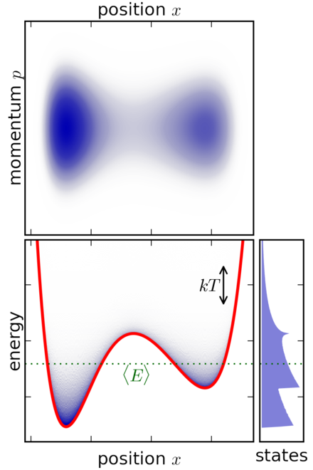
Figure 6: Example of canonical ensemble for a classical system with a particle in a potential well (source: Wikipedia)
Figure 6 shows a simple 1 dimensional classical (i.e., non-quantum) system where a particle is trapped inside a potential well. The system is submerged in a heat bath (not-shown) to keep it in thermal equilibrium. The top diagram shows the momentum vs. position, in other words it plots the phase space coordinates \((p, x)\). The bottom left plot shows the energy of the system vs. position with the red line indicating the potential energy at each \(x\) value. The bottom right plot shows the distribution of states across energy levels.
A few things to point out:
The particle moves along a single axis denoted by the position \(x\). So it essentially just moves left and right.
The velocity (or momentum) changes in two ways: (a) As it moves left and right, it gains or loses potential energy. This translates into kinetic energy affecting the velocity (and momentum). As it approaches an potential "uphill" its movement along the 1D axis slows in that direction, similarly when on a potential "downhill" its movement speeds up along the 1D axis in that direction. (b) The heat bath will be constantly exchanging energy with the system, which translates to changing the momentum of the particle. This happens randomly as a function of the equilibrium temperature.
The top phase space plot clearly shows the particle spending most of its paths (blue) in the dips in the potential function with varying momentum values. This is as expected because the particle will get "pulled" into the dips while the momentum could vary by the interaction with the heat bath.
The bottom left plot shows something similar where the particle is more concentrated in the dips of the potential function. Additionally, most of the time the internal system energy is close to the green dotted line, which represents the average energy of the particle system.
The bottom right plot shows the distribution of states by energy. Note that the energy states are not a simple exponential distribution as you may think from Equation 38. The distribution in Equation 38 is a function of the microstates \((q, p)\), not the internal system energy. This is hidden in the normalization constant \(Z\), which sums over all microstates to normalize the probabilities to 1. As a result, the distribution over energy states can be quite complex as shown.
As we can see from Equation 38 and Example 4, we have related the Hamiltonian to a probability distribution. We now (finally!) have everything we need to setup the HMC method.
This whole digression into thermodynamics is not for naught! We are in fact going to use the canonical ensemble to model and sample from our target distribution. Here's the setup for target density (or something proportional to it) \(f({\bf x})\) with \(D\) variables in its support:
Position variables (\(q\)): The \(D\) variables of our target distribution (the one we want to sample from) will correspond to our position variables \(\bf q\). Instead of our canonical distribution existing in (usually) 3 dimensions for a physical system, we'll be using \(D\) position dimensions for HMC.
Momentum variables (\(p\)): \(D\) corresponding momentum variables will be introduced artificially in order for the Hamiltonian dynamics to operate. They will allow us to simulate both the particle moving around as well as the random changes in direction that occur when it interacts with the heat bath.
-
Potential energy (\(U(q)\)): The potential energy will be the negative logarithm of our target density (up to a normalizing constant):
\begin{equation*} U({\bf q}) = -log[f({\bf q})] \tag{39} \end{equation*} -
Kinetic energy (\(K(p)\)): There can be many choices in how to define the kinetic energy, but the current practice is to assume that it is independent of \(q\), and quadratic in each of the dimensions. This naturally translates to a zero-mean multivariate Gaussian (see below) with independent variances \(m_i\). This produces the kinetic energy:
\begin{equation*} K({\bf p}) = \sum_{i=1}^D \frac{p_i^2}{2m_i} \tag{40} \end{equation*} -
Hamiltonian (\(H({\bf q, p})\)): Equation 39 and 40 give us this Hamiltonian:
\begin{equation*} H({\bf q, p}) = -log[f({\bf q})] + \sum_{i=1}^D \frac{p_i^2}{2m_i} \tag{41} \end{equation*} -
Canonical distribution (\(P({\bf q, p})\)): The canonical ensemble yields the Boltzmann equation from Equation 38 where we will set \(kT=1\) and plug in our Hamiltonian from Equation 41:
\begin{align*} P({\bf q, p}) &= \frac{1}{Z}\exp(\frac{H({\bf q, p})}{kT}) && \text{set } kT=1\\ &= \frac{1}{Z}\exp(-log[f({\bf q})] + \sum_{i=1}^D \frac{p_i^2}{2m_i}) \\ &= \frac{1}{Z_1}\exp(-log[f({\bf q})])\cdot\frac{1}{Z_2}\exp(\sum_{i=1}^D \frac{p_i^2}{2m_i}) \\ &= P(q)P(p) \tag{42} \end{align*}
where \(Z_1, Z_2\) are normalizing constants, and \(P(q), P(p)\) are independent distributions involving only those variables. Taking a closer look at those two distributions, we have:
So our canonical distribution is made up of two independent parts: our target distribution and some zero mean independent Gaussians! So how does this help us? Recall that the canonical distribution models the distribution of microstates (\(\bf q,p\)). So if we can exactly simulate the dynamics of the system (via the Hamilton's equations + random interactions with the heat bath), we would essentially be simulating exactly \(P({\bf q,p})\), which leads us directly to simulating \(P({\bf q})\)!
In this hypothetical scenario, we would just need to simulate this system, record our \(q\) values, and out would pop samples of our target distribution. Unfortunately, this is not possible. The main reason is that we cannot exactly simulate this system because, in general, Hamilton's equations do not yield a closed form solution. So we'll have to discretize Hamiltoninan dynamics and add in a Metropolis-Hastings update step to make sure we're faithfully simulating our target distribution. The next subsection describes the HMC algorithm in more detail.
3.2 HMC Algorithm
The core part of the HMC algorithm follows essentially the same structure as the Metropolis-Hastings algorithm: propose a new sample, accept with some probability. The difference is that Hamiltonian dynamics are used to find a new proposal sample, and the acceptance criteria is simplified because of a symmetric proposal distribution. Here's a run-down of the major steps:
Draw a new value of \(p\) from our zero mean Gaussian. This simulates a random interaction with the heat bath.
Starting in state \((q,p)\), run Hamiltonian dynamics for \(L\) steps with step size \(\epsilon\) using the Leapfrog method presented in Section 2.5. \(L\) and \(\epsilon\) are hyperparameters of the algorithm. This simulates the particle moving without interactions with the heat bath.
After running \(L\) steps, negate the momentum variables, giving a proposed state of \((q^*, p^*)\). The negation makes the proposal distribution symmetric i.e. if we run \(L\) steps again, we get back to the original state. The negation is necessary for our MCMC proof below but the negation is unimportant because we always square the momentum before using it in the Hamiltonian.
-
The proposed state \((q^*, p^*)\) is accepted as the next state using a Metropolis-Hastings update with probability:
\begin{align*} A(q^*, p^*) &= \min\big[1, \frac{f(q^*, p^*)g(q, p | q^*, p^*)}{f(q, p)g(q^*, p^* | q, p)}\big] \\ &= \min\big[1, \frac{f(q^*, p^*)}{f(q, p)}\big] && \text{symmetry of proposal distribution} \\ &= \min[1, \frac{\exp(-H(q^*, p^*))}{\exp(-H(q,p))}] \\ &= \min[1, \exp(-U(q^*) + U(q) -K(p^*)+K(p))] \\ \tag{44} \end{align*}If the next state is not accepted (i.e. rejected), then the current state becomes the next state. This MH step is needed to offset the approximation of our discretized Hamiltonian. If we could exactly simulate Hamiltonian dynamics this acceptance probability would be exactly \(1\) because the Hamiltonian is conserved (i.e. constant).
It's all relatively straight forward (assuming you have the requisite background knowledge above). It generally converges faster than a random walk-based MH algorithm, but it does have some key assumptions. First, we can only sample from continuous distributions on \(\mathcal{R}^D\) because otherwise our Hamiltonian dynamics could not operate. Second, similar to MH, we need to be able to evaluate the density up to a normalizing constant. Finally, we must be able to compute the partial derivative of the log density in order to compute Hamilton's equations. Thus, these derivatives must exist everywhere the density is non-zero. There are several other detailed assumptions you can look up in [1] if you are interested.
What's nice is that all that math reduces down to quite a simple algorithm. Listing 1 shows pseudo-code for one iteration of the algorithm, which is pretty straightforward to implement (see the experiments section where I implement a toy version of HMC).
Listing 1: Hamiltonian Monte Carlo Python-like Pseudocode
Listing 1 is a straight forward implementation of Leapfrog combined with a simple acceptance step. An optimization is done on line 23 to combine the two half momentum steps from Equation 35 and 37. A bit of the magic is hidden behind the potential and gradient of the potential function but those depend fully on your target distribution so it can't be helped.
It's not obvious that the above algorithm would be correct, particularly the acceptance step, which we simply stated without much reasoning. We'll examine its correctness the next subsection.
3.3 HMC Algorithm Correctness
To show that HMC correctly produces samples, we will show that the algorithm correctly samples from the joint canonical ensemble distribution \(P(q, p)\). Since we already identified that this joint distribution can be factored into independent distributions \(P(q)\) and \(P(p)\) (Equation 42), our final output can just take the \(q\) samples to get our desired result.
We ultimately want to show that the next state returned in Listing 1 occurs with the correct probability according to the canonical distribution. First, we'll look at the very first operation: sampling of the momentum (Line 11 from Listing 1). Assume that you have sampled \(q\) properly (up to this point) according to our canonical distribution (the input to Listing 1). Since our momentum factor is independent, we can simply sample the momentum from its correct distribution (an independent normal distribution) and the resulting sample \((q, p)\) will distributed according to the canonical ensemble as required.
Next, we'll look at the rest of the algorithm, which runs Leapfrog for L steps and does an MH update (Line 15-41). We'll only be sketching the idea here and will not go into too many formalities. To start, let's divide up phase space (\((q, p)\)) into arbitrarily small partitions. Since these are arbitrarily small regions, the probability density, Hamiltonian and other associated quantities are constant within those region. The idea is that these finite regions can be shrunk down to infinitesimally small sizes that we would need to prove the general result. Additionally, this is where the volume-preserving nature of the Leapfrog algorithm comes in (and negation of the momentum, which is also volume-preserving). We don't need to worry about our small regions ever growing (or shrinking) and thus, we can treat any region (before or after a Leapfrog step) similarly.
Assume you have sampled the current state \((q, p)\) according to the
canonical distribution i.e., \((q, p)\) after you sample the momentum.
The probability that the next state is in some (infinitesimally) small region
\(X_k\) is the sum of probabilities that it's (a) already in \(X_k\) and it gets rejected
(else statement in Listing 1) plus (b) the probability that it's in some other state
and moves into state \(X_k\). Given canonical distribution probability state
\(P(X_k)\), rejection probability \(R(X_k)\), and
transition probability \(T(X_k|X_i)\) from region \(i\) to \(k\),
we can see that:
Thus, we see that our procedure will have correctly sampled our next state \(X_k\) according to the target distribution. From the second line, detailed balance (aka reversibility) is one of the key properties that we must have for this to work properly. The other thing to notice is that the probability of leaving state \(X_k\) to any given state is precisely the probability of not rejecting. So if we satisfy detailed balance (and the Markov chain has a steady state), we will have shown that we correctly sampled from the canonical distribution.
Now we will show the three conditions needed for a Markov chain described in the background to show that it does converge to a steady state and has the detailed balance condition. First, our procedure trivially can reach any state due to the normally distributed momentums, which span the real line, thus it is irreducible (practically though it is critically important to tune the variance on the normal distributions due to finite runs). Second, we need to ensure that the system never returns to the same state with a fixed period (i.e., it is aperiodic). Theoretically, this may be possible in certain setups but can be avoided by randomly choosing \(\epsilon\) or \(L\) within a narrow interval. Practically though, this is pretty rare on any non-trivial problem, although this may lead to other problems like very slow to converge.
Lastly, all that is left to show is that detailed balance is satisfied. Assume we start our Leapfrog operation in state \(X_k\) and run it for \(L\) steps plus reverse the momentum, and end in state \(Y_k\). We need to show detailed balance holds for all \(i,j\) such that:
Let's break it down into two cases:
Case 1 \(i \neq j\): Recall that the Leapfrog algorithm is deterministic, therefore \(Y_i = \text{Leapfrog_Plus_Reverse}(X_i)\) for any given \(k\). So if you have any other \(Y_{j\neq i}\) then it is impossible to transition to this state. Thus, \(T(X_i|y_j) = 0\) and Equation 46 is trivially satisfied.
Case 2 \(i = j\): In this case, let's plug in our transition/acceptance probability condition (Equation 44) and see what happens. Note that in addition to the probability being constant within a region, we also have the Hamiltonian constant too. Let \(V\) be the volume of the region, \(H_{X_k}, H_{Y_k}\) be the value of the Hamiltonian in each region, and without loss of generality assume \(H_{X_k} > H_{Y_k}\) (due to symmetry of the problem). Plugging this all into Equation 46, we see that it satisfies the detailed balance condition:
where the probability of being in state \(P(X_i)\) is the volume of the region (\(V\)) multiplied by the density (Boltzman distribution). This works because of our infinitesimally small regions where we assume the density is constant throughout.
Two subtle points to mention. First, if we were able to simulate Hamiltonian dynamics exactly, \(H_{X_k} = H_{Y_k}\) (recall the Hamiltonian is constant along a trajectory), then that would get us to a 100% acceptance rate. Unfortunately, Leapfrog or any other approximation method doesn't quite get us there so we need the MH step. Second, the reason why we need to negate the momentum at the end is so that our transition probabilities are symmetric, i.e. \(T(X_k|Y_k) = T(Y_k|X_k)\) (Equation 44), which follows from the fact that we can reverse our Leapfrog steps by negating the momentum and running it back the same number of steps. If we didn't include this step, then we would have to include another adjustment factor (\(g(y|x) / g(x|y)\)), which comes from the more generic MH step described in Equation 1.
3.4 Additional Notes
It should be pretty obvious that the explanation above only presents the core math behind HMC. To make it practically work, there are a lot more details. Here are just a few of the issues that make a real world implementation complex (for all these points, [1] has some additional discussion if you want more detail):
Tuning step size (\(\epsilon\)) and number of steps (\(L\)) is so critically important that it can make or break your HMC implementation (see discussion in the experiments below). You can get into all sorts of incorrect sampling behaviors if you get it wrong from highly correlated samples to low acceptance rates. You have to be very careful!
Similarly, tuning the momentum hyperparameters (the standard deviation for our independent Gaussians in our case) is also very important to getting proper samples. If your momentum is too low, then you won't be able to explore the tails of your distribution. If your momentum is too high, then you'll have a very low acceptance rate. To add to the complexity, the momentum distribution is related to the step size and number of steps too. In general, it's best if you can tune each dimension of the momentum distribution to fit your problem but that is typically non-trivial.
In general, you'll have a mix of discrete and continuous variables. In those cases, you can mix and match MCMC methods and use HMC only for a subset of continuous variables. Similarly, there are adaptations of HMC to continuous variables that don't span the real line.
A practical technique to use HMC was the discovery of the No U-Turn Sampler (NUTS). Roughly, the algorithm adaptively sets the path length by running Leapfrog both backwards and forwards in time, and then seeing where the trajectory "changes direction" (a "U-Turn"). At this point, you randomly sample a point from your path. In this way, you likely have seen enough of the local landscape to not double back on your path (which wastes computation) but still have enough momentum to reach the tails. As far as I can tell, most implementations of HMC will have a NUTS sampler.
4 Experiments
As usual, I implemented a toy version of HMC to better understand how it works. You can take a look at the code on Github (note: I didn't spend much time cleaning up the code). It's a pretty simple implementation of HMC and MH MCMC algorithms, which pretty much mirrors the pseudocode above.
I ran it for two very simple examples. The first is a standard normal distribution, where you can see the run summary in Figure 7. The two left and two right panels show the HMC and MH results, respectively. Both methods use a standard normal distribution for the momentum distribution and the proposal distribution, respectively. I show the histogram of 1000 samples (overlaid with the actual density) with its associated autocorrelation plot. You can see that the HMC algorithm has a higher acceptance rate (97% vs. 70%), which results in fewer steps needed to sample.
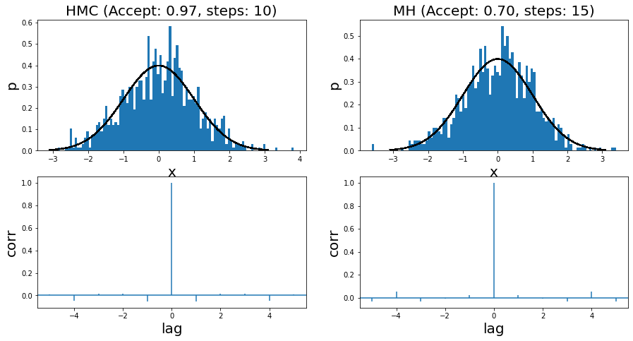
Figure 7: Histogram of samples from toy implementation of HMC and MH for a standard normal distribution
Overall the samples look more or less reasonable. This is backed up by the autocorrelation (AC) plots, which shows little to no correlation between samples (i.e. independence). I had to (manually) tune both algorithms in order to get to a point where the AC plots didn't show significant correlation. For MH, I had to increase the step size sufficiently. For HMC, I had to tune between the step size and number of steps to get that result.
Adding another dimension, I also ran HMC and MH for a bivariate normal distribution with standard deviation in both dimension of \(1.0\), and a correlation of \(0.9\) for 1000 samples. The samples are plotted (from left to right, top to bottom) in Figure 8 for two HMC runs, a MH run, and directly sampling from the distribution (via Numpy). I plotted the unit circle to give a sense of scale of the standard deviation of two dimensions (multivariate normal distributions with non-diagonal covariance matrices don't typically look spherical though). I also tuned all of them (except for Numpy) to have a relatively low autocorrelation plot. In the plot titles, "Acc" stands for acceptance rate, "eps" is epsilon, "st" is steps, "pstd" is standard deviation for momentum normal distribution (same for both dimensions), "prop" is proposal distribution (same standard deviation for both dimensions).
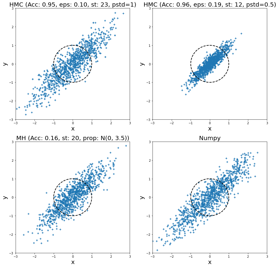
Figure 8: Histogram of samples from toy implementation of HMC, MH, and Numpy for a bivariate normal distribution
Looking at the top left HMC samples and the bottom right Numpy direct sampling, we can see they are visually very similar. This is a good case of being able to generate reasonable samples. I ran another HMC example but with a smaller standard deviation (top right), and you can see all the samples are concentrated in the middle. This shows that setting the momentum properly is critical for generating proper samples. In this case, we see that the distribution doesn't have enough "energy" to reach far away points so we never sample from there (for this particular finite run).
Turning to the MH sampler, visually it also looks relatively similar to the Numpy samples. Similar to HMC, I had to set the standard deviation of the proposal distribution (independent Gaussians) to a relatively large value. If not, then it would be extremely unlikely to reach distant points (unless you had many more steps). The large random jumps result in a very low acceptance rate, which means we need more proposal jumps to get independent samples.
I considered doing a more complex example such as a Bayesian linear regression or hierarchical model, but after all the fiddling with the two simple examples above, I thought it wasn't worth it. I'll leave the MCMC implementations to the pros. I'm already quite satisfied with the understanding that I've gained going through this exercise (not to mention my newfound appreciation for its complexity) .
5 Conclusion
It's really rewarding to finally understand (to a satisfactory degree) a topic that you thought was "too difficult" just a few years ago. I originally wasn't looking to do a post on HMC but went down this rabbit hole trying to understand another topic that slightly overlaps with it. This is part of the joy of being able to independently study things, too bad time is so limited. In any case, I'm hoping to eventually get back to the topic that I was originally interested in at some point, and hopefully be able to find time to post more often. In the meantime, stay safe and have a happy holidays!
6 Further Reading
Previous posts: Markov Chain Monte Carlo Methods, Rejection Sampling and the Metropolis-Hastings Algorithm, The Calculus of Variations
Wikipedia: Metropolis-Hastings Algorithm, Classical Mechanics, Lagrangian Mechanics, Hamiltonian Mechanics
[1] Radford M. Neal, MCMC Using Hamiltonian dynamics, arXiv:1206.1901, 2012.
[2] David Morin, Introduction to Classical Mechanics, 2008.
[3] HyperPhysics
- 1
-
The usual symbols they use for the Lagrangian are \(L = T - U\) representing the kinetic and potential energy respectively. However, \(T\) makes no sense to me, so since we're not really talking about physics here, I'll just use \(K\) to make it clear for the rest of us.
- 2
-
This physical analogy is not exactly accurate because gravity, which affects the velocity of the puck, doesn't quite match our target density. Instead, a better analogy would be a particle moving around in a vector field (e.g. an electron moving around in an electric field defined by our target density). Although more accurate, it's less intuitive than a puck sliding along a surface so I get why the other analogy is better.