A Variational Autoencoder on the SVHN dataset
In this post, I'm going to share some notes on implementing a variational autoencoder (VAE) on the Street View House Numbers (SVHN) dataset. My last post on variational autoencoders showed a simple example on the MNIST dataset but because it was so simple I thought I might have missed some of the subtler points of VAEs -- boy was I right! The fact that I'm not really a computer vision guy nor a deep learning guy didn't help either. Through this exercise, I picked up some of the basics in the "craft" of computer vision/deep learning area; there are a lot of subtle points that are easy to gloss over if you're just reading someone else's tutorial. I'll share with you some of the details in the math (that I initially got wrong) and also some of the implementation notes along with a notebook that I used to train the VAE. Please check out my previous post on variational autoencoders to get some background.
Update 2017-08-09: I actually found a bug in my original code where I was only using a small subset of the data! I fixed it up in the notebooks and I've added some inline comments below to say what I've changed. For the most part, things have stayed the same but the generated images are a bit blurry because the dataset isn't so easy anymore.
The Street View House Numbers (SVHN) Dataset
The SVHN is a real-world image dataset with over 600,000 digits coming from natural scene images (i.e. Google Street View images). It has two formats: format 1 contains the full image with meta information about the bounding boxes, while format 2 contains just the cropped digits in 32x32 RGB format. It has the same idea as the MNIST dataset but much more difficult because the images are of varying styles, colour and quality.
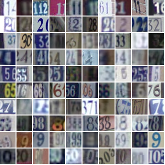
Figure 1: SVHN format 2 cropped digits
Figure 1 shows a sample of the cropped digits from the SVHN website. You can see that you get a huge variety of digits, making the it much harder to train a model. What's interesting is that in some of the images you have several digits. For example, "112" in the top row, is centred (and tagged) as "1" but has additional digits that might cause problems when fitting a model.
A Quick Recap on VAEs
Recall a variational autoencoder consists of two parts: a generative model (the decoder network) and the approximate posterior (the encoder network) with the latent variables sitting as the connection point between the two.
Writing the model out more formally, we have this for the generative model which takes a latent variables \(Z\) and generates a data sample \(X\):
To help fitting, we want to generate (an approximate) posterior distribution for \(Z\) given a \(X\):
Check out my previous post on this topic for more details and intuition. Figure 2 shows an illustration of a typical variational autoencoder.
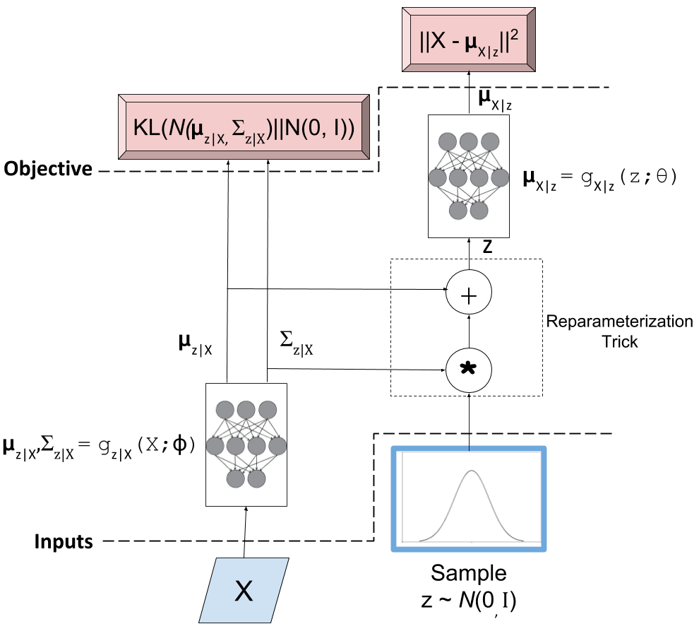
Figure 2: A typical variational autoencoder
The key point for this discussion are the two objective functions (i.e. loss functions). The left hand side loss function is the KL divergence which basically ensures that our encoder network is actually generating values that match our prior \(Z\) (a standard isotropic Gaussian). The right hand side loss is the log-likelihood of observing \(X\) for our given output distribution with parameters generated by our decoder network. We want to minimize the sum of both loss functions to ensure that our generative model works. That is, we can sample our \(Z\) values from a standard isotropic Gaussian and our network will faithfully generate sample that are close to the distribution of \(X\).
Fixed or Fitted Variance?
One subtlety that I glossed over in my previous post was the output distribution on \(X\). Whenever I referenced the output variable, I assumed it was a continuous normal distribution. However, for the MNIST example that I put together, the output variable was a Bernoulli. Note that although each \(X_i\) is actually a discrete pixel value (say between 0 and 255), we can still conveniently model it as a Bernoulli by normalizing it between 0 and 1. This is not exactly proper since a Bernoulli only has 0/1 values but it works well in practice.
Let's take a look at what that looks like by taking the log-likelihood of the output variable:
which is just the cross entropy between \(X\) and \(p\), where \(K\) is the length of \(X\) and \(p\). This is precisely the output loss function that we used in the notebook. Note that in this case \(X\) is our observed value (i.e. MNIST image that we train on) and \(p\) is the value that our decoder network generates (the analogue to \(\mu_{X|z}\) above).
Let's try the same thing with a normal distribution as our output variable (we'll treat each part of \(X\) as independent since we're assuming a diagonal covariance matrix):
Again, remember that \(X\) values are our observed values (e.g. our image) and \(\mu_i, \sigma_i^2\) is what our fitted neural network is going to produce.
The big question here is what to do with \(\sigma^2\)? In Doersch's tutorial (see references below), he sets \(\sigma_i^2\) to a constant hyperparameter that is the same across all dimensions of \(X\) 1. But if you think about, why should the variance be the same across all dimensions? For example, the top left corner of an image might always be a dark pixel so its variance would be small. In contrast, a pixel in the center might be very different from image to image so it would have a high variance. For many cases, it doesn't quite make sense to set the variance to a constant hyperparameter across all pixels.
This was initially a big roadblock for me because I was primarily following Doersch's tutorial. However, one of the original VAE papers by Kingma (see references below) explicitly models each \(\sigma_i^2\) separately as another output of their decoder network. In one Kingma's later papers, he uses a VAE for comparison on the SVHN dataset and even has an implementation! Had I just looked at it sooner, it would have been much easier. However, this wasn't the only misunderstanding that I had.
Modelling \(\sigma^2\)
A couple of notes on implementing a loss function with \(\sigma^2\). I had a lot of trouble implementing Equation 4 as Kingma did in his paper. His decoder network outputs two values: the mean \(\mu_i\) and log-variance \(u:=\log\sigma^2\). He uses a standard dense fully connected layer for both with no activation function. This allows both values to range from \((-\infty, \infty)\). However, notice how Equation 4 changes with this change of variables:
You're now dividing by an exponential in the last term. If the denominator gets anywhere close to \(0\), your loss function blows up. I've seen more "nan"'s in this project than all my other work with other types of models :p
One solution to this problem is an idea I found in a Reddit thread (after much trial and error). Basically, we can model \(\sigma^2\) directly plus an epsilon to ensure that it doesn't blow up. So we define the output of our network as \(v:=\sigma^2 + \epsilon\) and use a "ReLU" activation function to ensure that we only get positive numbers. Let's take a look at this new change of variables:
\(\epsilon\) is a hyperparameter that needs to be small enough to be able to capture the variance of your smallest dimension (bigger variances can be generated by the "ReLU" function). Along with this issue, you have to make sure that you're learning rate is small enough to allow your loss function to converge because we're still dividing by potentially small values that can vary widely 2.
BK : I actually was playing around with Kingma's method and I did get it to not blow up by using a combination of the initialization of weights on the variance output nodes and putting L2 regularization on it to keep it small. It's still actually a bit tricky because if your learning rate is too small, the weights will not deviate that far from your initialization, which might not give you a small enough variance. I didn't try to get it working fully but I may try it in my next model.
A Digression on Progress
As an aside, I'm still find it quite astounding that I am able to reproduce state of the art research from only a few years back (2014) so quickly. If I had known what I was doing at the start, I probably could have put it together in a few hours or so. The pervasiveness of deep learning frameworks is incredible. Using open source frameworks like Keras, you can probably train most network architectures that took a grad student months to code just a few years ago. Not only that, we have incredibly powerful GPUs that are an order of magnitude more powerful than anything available around that time. Both these things have accelerated the deep learning wave, and definitely are huge contributors to its progress.
Now I'm not the type of person who says deep learning is the hammer that can be applied to every problem (there are many situations for which deep learning is not appropriate) but you have to admit, the progress we have seen, the problems it is solving, and the promise it brings, is pretty incredible. So anyways, with this topic I'm going to start investigating the parts of deep learning that I find interesting (especially ones that have a more solid probabilistic basis) and see where it takes me. Back to our regularly scheduled program.
Convolution or Components?
One of the first things I tried was just to adapt the example network from Keras that I showed in my previous post and use it verbatim to train the SVHN dataset. It didn't work very well. The network uses convolution layers and transpose convolution layers for the encoder/decoder networks respectively. One of the issues that I kept getting was that the loss would bottom out at a poor fit. All I would get in the end was a bunch of blurry images with something that looked like "3" or an "8", nothing too impressive.
I tried and failed for quite a while to get a CNN to fit properly but didn't get anywhere with it. Some of the things I tried:
Adding more or less convolutional layers (between 3-8) on each encoder/decoder
Adding more or less dense layers to encode the latent variables
Changing the stride of the convolutional layers higher or lower
Using an identical architecture on the decoder to a generative adversarial network
Nothing would quite work. After searching the web for a while, I finally came across this Reddit post with someone who was trying to solve exactly the same problem. The advice was basically to use the "PCA trick", which was to use principal component analysis and then fit a non-convolutional variational autoencoder (i.e. only use fully connected layers). Here someone mentioned that Kingma's has his code for one of his later papers in which he compared his method to a standard variational autoencoder on the SVHN dataset.
After many iterations of tweaking the model, reading up on PCA, and reading Kingma's code (it was written in Theano so not as easy to read as high level APIs like Keras), I was finally able to get PCA to work with the breakthrough being the correct modelling of the variance, per dimension, as described in the previous section. As to why PCA seems to work, here's what I gathered:
PCA transforms the RGB image into the \(K \leq N\) dimensions, where \(N\) is the original dimension of the image (e.g. For SVHN: 32x32x3 = 3072). In detail, we're rotating the data into an orthogonal basis defined by the eigenvectors of its covariance matrix. The result it that the dimensions defined by the first \(K\) eigenvectors define most of the covariability of the data (in proportion to their eigenvalues). In simple terms, we capture most of the signal in the data just by taking the top principal components.
Using a number a bit higher than Kingma (\(K=1000\) vs \(600\)), I was able to reduce dimensionality of the images without much corruption (there were a few occasional patches of image with discoloration but nothing major). This indicates there is a lot "noise" that we can throw away that is not really relevant to the actual "signal" of the image. BK : I actually changed this down to K=500 without much loss in quality to the naked eye. The corruption I was getting was simply due to a bit of precision loss when converting to/from PCA dimension and some pixels were getting an invalid value (e.g. > 255), after clipping to a valid range there was no more visible corruption.
The components have large magnitude differences (another reason for per-dimension variances), with the first principal component being the largest.
Due to the PCA transformation, the loss function could pay more "attention" to the largest principal component and capture more of the variance (i.e. signal) because the squared error term from this component would be huge if it were off even by a bit.
However, after a while the loss function would also be able to find good weights for even the smallest component by scaling the variance appropriately, making sure we capture the "detail" specified in these smaller components.
Note: I couldn't get it to work with PCA whitening, where the PCA components are scaled to have unit variance. I suspect it's because of this dynamic between different magnitudes, it doesn't "focus" the loss function well on the principal component and treats all components equally (perhaps this would work well with a constant variance?). This could be another issue with the learning rate though, I didn't spend too much time going back to investigate.
In any case, fitting a variational autoencoder on a non-trivial dataset still required a few "tricks" like this PCA encoding.
Implementation Notes
Here are some odds and ends about the implementation that I want to mention. The actual implementation is in these notebooks. Some of these things are obvious to a seasoned deep learning expert but may help novices like me who are still learning about the "art" of fitting deep models.
For the fully connected dense layers, I added batch normalization before the activation, followed by a "ReLU" activation, followed by a dropout layer. I did this because it seems to be the consensus for best practice: batch norm and "ReLU" seem to speed up convergence and avoid the gradients from blowing up, and dropout to ensure that when we use huge networks we don't overfit. I didn't try many alternatives (like a traditional sigmoid or "tanh" activation), although when playing doing the MNIST dataset I did have some problems (exploding gradients) deep nets without batch norm and "ReLU", so it's likely they were necessary.
I didn't really tune the dropout, which was set at \(0.4\) simply because I saw it used in someone else's post of variational autoencoders. I just assumed that if my network was big enough, a big dropout wouldn't really matter. BK : Arbitrarily changed it to 0.2 so the loss would converge a bit faster (wouldn't jump around so much in the beginning).
I followed the advice from the Stanford CNN course, which says to favour bigger networks with regularization instead of using smaller networks to prevent overfitting. I ended up using 512 latent variables, and 5 dense layers on the encoder with 2048 neurons, and (roughly) 6-7 layers on the output for the mean and variance respectively. Somehow it seems a bit of overkill but again it's easier to find good fits on bigger networks so I didn't want to spend that much time searching for a smaller network size.
To speed up the iterations a bit, I used a bigger batch size (1000). This was pretty arbitrary but I suppose I should increase it to the biggest batch size that can fit on my GPU. This is because the network it loads onto your GPU is actually batch_size * network size, and it does batch_size back-propagations in parallel and averages their gradients. Naturally, if batch_size is bigger, it will run faster because it works in parallel (so as long it fits on your GPU). BK : I actually tried increasing the batch size to 6300 with worse results! See this SO answer. Basically the reasoning is that since the gradient is an approximation, you don't want to use too big of a batch or else you find local minima that are "sharp", whereas smaller batches converge to "flat" ones. The "flat" parts of the objective function are probably where you want to be instead of spurious "sharp" ones. In my case, I converged to a loss of around -150 or so with a 6300 batch size but was able to get to around -250 with a batch of 1000. So bigger is not always better! Definitely some trade-off though because batch size of 1 would converge too slowly.
On a related note, this would basically be impossible without a GPU. The fitting time would be ridiculous, which again is a testament to the advancements in computational power.
I used a large number of epochs (1000) with a stopping condition on the training loss (not validation loss). Interestingly, for this application I think we might want to "overfit" so we can memorize the distribution of the input images using our generative model (i.e. decoder network). This should produce images that are closer to the real thing. I tried an early stopping condition on the validation loss and it stopped prematurely causing a lot of blurriness in the images. For other applications such as semi-supervised learning, where you use the encoder network to map your input to a latent variable space, you probably do want to stop on validation loss. Interestingly, I don't think that is the case here (please let me know if I'm wrong!). BK : Changed this to 2000 epochs but it started learning so slowly after 1000 or so that I probably could've stopped then.
As mentioned above, I lowered learning rate to 0.0001 using the "Adam" optimizer. The optimizer choice was arbitrary, I saw it used somewhere else so I also used it. The learning rate was key, especially as I lowered the \(\epsilon\) lower bound on the variance, otherwise the gradient would jump around like crazy and eventually blow up (i.e. "nan" loss).
Initially, I only used a randomly selected 20% of the SVHN dataset to train in order to speed my iterations up. I couldn't get good results, so I eventually bumped it up to just about the entire dataset (rounded to be my batch_size to make the math easier). Probably training with more data resulted in a better fit but I strongly suspect the reason I'm able to fit now is the PCA + variance trick. I've been too lazy to go back to see if this contributed to the cause of my poor fits.
To be able to fit the entire dataset, I had to use Keras fit_generator() API so that I could fit everything in memory. I setup a generator that returns the next batch_size of images with PCA applied on the fly. The generator then cycles through the entire dataset indefinitely, which is what the Keras API expects. Probably if I was a bit more careful, I could perform the PCA in memory without overloading my 16GB of RAM but I was a bit lazy and didn't want to do any optimization. Alternatively, I'm sure I could of preprocessed everything with PCA and then saved the resulting PCA-transformed images.
Keep in mind, to recover an human-interpretable image on the output of the network you have to apply the inverse transform of your PCA model. Keras' own image processing API has a ZCA operation but no inverse, so I just ended up using Scikit's implementation, which has an nice API for inverting the PCA-transform.
A small note on implementing the loss function: the tensor (i.e. multi-dimensional array) that is passed into the loss function is of dimension batch_size * data_size. So for our 1000 dimension PCA transformed output with batch size 1000, we would have a tensor of 1000x1000. So when computing the loss, you want to perform the loss on each 1000 dimension slice of the tensor, and then average over your entire batch. Keep this in mind when you're doing operations (which need the Keras specific versions so it knows how to compute the gradient) and make sure you're performing it across the right axis. Checkout my implementation for some examples.
Variational Autoencoder SVHN Results
After all of that work, we can finally see something interesting! I've uploaded a few notebooks that contain my implementation to Github so you can try to run it yourself (let me know if you find a bug or improvement!). Figure 3 shows 100 randomly sampled images from our generator network:
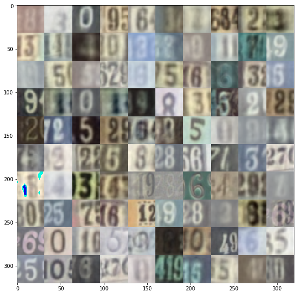
Figure 3: Images randomly generated from our variational autoencoder generator network
A bit blurry but remember the originals were also a bit blurry :p Actually it's somehow common knowledge that VAEs produce blurry images (at least compared to GANs). What's cool is that we get quite a variety of digits, styles, colours that are sampled just from our generator network! It's even more surprising that the network was able to learn "complex" images, ones where there are multiple digits in the picture. BK : The updated images are blurrier than this one, although you can definitely make out all the numbers still. The entire SVHN dataset is much harder! Check out the notebook for the updated images.
Next, let's try some analogies where we run a image from our original dataset through the entire VAE network and see some "analogies". These analogies are sampled from the latent variable space that our network are learned. Figure 4 shows some analogies for digits 0-9. The images in the first column are the originals, the rest of the row are images we've generated by sampling.
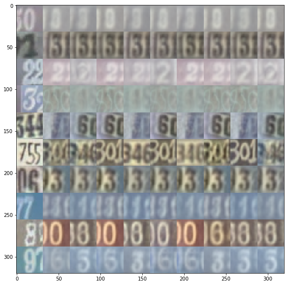
Figure 4: Images analogies randomly generated from using our entire variational autoencoder network
The analogies aren't exactly what I thought they would be. I was expecting to see rows of "1"s, "2"s etc. or even similar colours and styles across the rows. Some have similarities (in terms of colour or number), while others seem way off. It's kind of hard to tell if we're doing the right thing because we've transformed into PCA space, so it's much harder to interpret what's going on. BK : After training with the entire dataset, the analogies look a lot better! They are actually very close to the given image in terms of colour and sometimes number. Check out the notebook for the updated images.
Additionally, I suspect the way I've encoded the output variance allows a "generous" deviation from the actual source image, perhaps resulting in the wide variation. If you have some more insight, please let me know :)
Conclusion
It seems that non-trivial deep networks still require a bit of "art" to use. I can see why they've become so popular though, it's really fun to work with a dataset that you can literally see (i.e. images). I think it's so cool that the network I trained is able to generate realistic looking images. The math involved in VAEs is also really cool too (but probably I'm in the minority on this view). I'm going to keep exploring the VAE topic for a bit because I find it really interesting. Make sure to check back for future posts!
Further Reading
Previous Posts: variational autoencoders
Wikipedia: Cross Entropy
Relevant Reddit Posts: Gaussian observation VAE, Results on SVHN with Vanilla VAE?
"Tutorial on Variational Autoencoders", Carl Doersch, https://arxiv.org/abs/1606.05908
"Auto-Encoding Variational Bayes", Diederik P. Kingma, Max Welling, https://arxiv.org/abs/1312.6114
"Code for reproducing results of NIPS 2014 paper "Semi-Supervised Learning with Deep Generative Models", Diederik P. Kingma, https://github.com/dpkingma/nips14-ssl/
The Street View House Numbers (SVHN) Dataset, http://ufldl.stanford.edu/housenumbers/
CS231n: Convolutional Neural Networks for Visual Recognition, Stanford University, http://cs231n.github.io/neural-networks-1/
PCA Whitening - UFLDL Tutorial, Stanford University, http://ufldl.stanford.edu/tutorial/unsupervised/PCAWhitening/
"Batch Normalization: Accelerating Deep Network Training by Reducing Internal Covariate Shift", Sergey Ioffe, Christian Szegedy, https://arxiv.org/abs/1502.03167
- 1
-
I'm sure Doersch knows that this is not always the right thing to do. He probably was just trying to simplify the explanation in the tutorial to make the flow smoother.
- 2
-
I'm sure the learning rate and initialization of weights is somehow related to how Kingma's implementation works. I didn't really spend much time trying to figure this out after I got my implementation working though.